
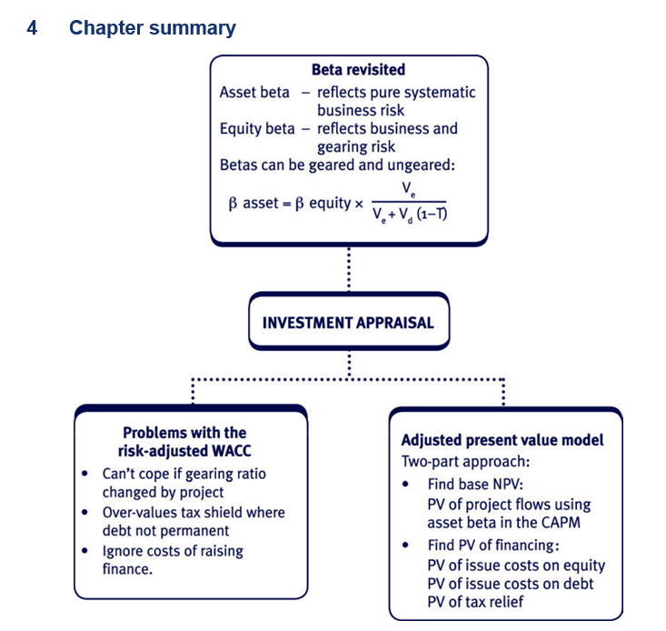
Introduction
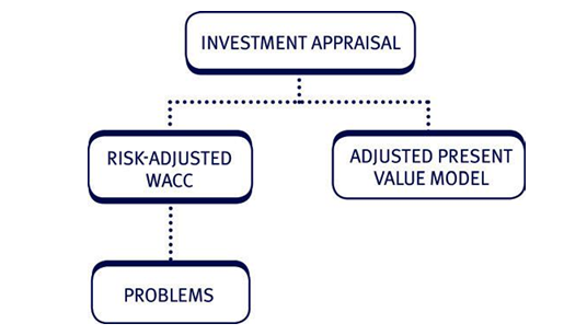
Alternatives to the use of existing WACC as a discount rate in project appraisal
We have now established that the existing WACC should only be used as a discount rate for a new investment project if the business risk and the capital structure (financial risk) are likely to stay constant. Alternatively,
If the business risk of the new project differs from the entity’s existing business risk
A risk adjusted WACC can be calculated, by recalculating the cost of equity to reflect the business risk of the new project. This often involves the technique of ‘degearing’ and ‘regearing’ beta factors, covered later in this chapter.
If the capital structure (financial risk) is expected to change when the new project is undertaken
The simplest way of incorporating a change in capital structure is to recalculate the WACC using the new capital structure weightings. This is appropriate when the change in capital structure is not significant, or if the new investment project can be effectively treated as a new business, with its own long term gearing level.
Alternatively, if the capital structure is expected to change significantly, the Adjusted Present Value method of project appraisal could be used. This approach separates the investment element of the decision from the financing element and appraises them independently. APV is generally recommended when there are complex funding arrangements (e.g. subsidised loans).
The risk adjusted WACC
Basic principle
If the business risk of the new project is different from the business risk of a company’s existing operations, the company’s shareholders will expect a different return to compensate them for this new level of risk.
Hence, the appropriate WACC which should be used to discount the new project’s cash flows is not the company’s existing WACC, but a ‘risk adjusted’ WACC which incorporates this new required return to the shareholders (cost of equity).
Calculating a risk-adjusted WACC
- Find the appropriate equity beta from a suitable quoted company.
- Adjust the available equity beta to convert it to an asset beta – degear it.
- Readjust the asset beta to reflect the project (i.e. its own) gearing levels – regear the beta.
- Use this beta in the CAPM equation to find Ke.
- Use this Ke to find the WACC.
- Evaluate the project.
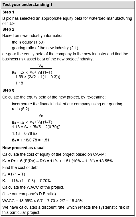
Test your understanding 1
B plc is a hot air balloon manufacturer whose equity:debt ratio is 5:2.
The company is considering a waterbed-manufacturing project. B plc will finance the project to maintain its existing capital structure.
S plc is a waterbed-manufacturing company. It has an equity beta of 1.59 and a Ve:Vd ratio of 2:1.
The yield on B plc’s debt, which is assumed to be risk free, is 11%. B plc’s equity beta is 1.10. The average return on the stock market is 16%. The corporation tax rate is 30%.
Required:
Calculate a suitable cost of capital to apply to the project.
Student Accountant articles
Read the pair of articles ‘Cost of capital, gearing and CAPM’ in the Technical Articles section of the ACCA website for more details on the risk adjusted WACC.
Using the risk-adjusted WACC
The risk-adjusted WACC calculated above reflects the business risk of the project and the current capital structure of the business, so it is wholly appropriate as a discount rate for the new project.
Two other issues also need to be considered:
- The method used to gear and degear betas is based on the assumption that debt is perpetual. This overvalues the tax shield where debt is finite.
- Issue costs on equity are ignored.
Theoretical points re: risk adjusted WACC
The degearing and regearing procedure is a product of the M&M 1963 position. To use these equations debt must be perpetual and risk free. If it is not perpetual, to ignore that it is for a shorter period will overvalue the tax shield on debt.
The value Ve + Vd used in the WACC equation should represent market values of debt and equity after the project has been adopted (i.e. the equity value should include the NPV of the project).
By using the ratio of the company before the project we have assumed that the project has a zero NPV – this is unlikely to be the case. If the project has a positive NPV the calculation will assume that borrowing is proportional to the present value of future cash flows rather than the initial value of the asset.
3 The adjusted present value (APV) technique
Basic principle
The APV method evaluates the project and the impact of financing separately. Hence, it can be used if a new project has a different financial risk (debt-equity ratio) from the company, i.e. the overall capital structure of the company changes.
APV consists of two different elements:
| APV | = | Base case NPV | + | Financing impact |
| (3) Value of a | = | (1) Value of an all | + | (2) Present value of |
| geared project | equity financed | financing side | ||
| project | effects |
The investment element (base case NPV)
The project is evaluated as though it were being undertaken by an all equity company with all financing side effects ignored. The financial risk is quantified later in the second part of the APV analysis. Therefore:
- ignore the financial risk in the investment decision process
- use a beta that reflects just the business risk, i.e. ß asset.
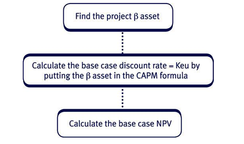
Once the base case NPV is identified, the PV of the financing package is evaluated.
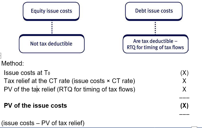
The financing impact
Financing cash flows consist of:
- issue costs
- tax reliefs.
As all financing cash flows are low risk they are discounted at either:
- the kd or
- the risk free rate.
Examples of exam tricks on APV
APV tricks
In exam questions, you may see the following tricks when calculating the ‘financing impact’ part. All these tricks are covered in the next ‘Test your understanding’ questions:
Grossing up
A firm will know how much finance is required for the investment. Issue costs of finance will usually be quoted on top. It will therefore be necessary to gross up the funds to be raised.
Grossing up illustration
The finance required for a planned investment is $2m (net of issue costs). Issue costs are 3%. And the finance raised will also have to cover the issue costs.
What are the issue costs and what sum will need to be raised altogether?
Solution
The $2m is 97% of the amount to be raised:
Therefore, ($2m/0.97) = $2,061,856 will be needed.
Issue costs are 3%
3% × $2,061,856 = $61,856
Issue costs can be calculated in one stage as:
$2m × 3/97 = $61,856
PV of debt issue costs
As always, calculations involving debt must take account of the tax effects.
PV of the tax relief on interest payments
The PV of the tax relief on interest payments is also known as the PV of the tax shield.
The method adopted depends on the information given:
Simple scenario: Bonds – interest paid at a fixed amount each year
Annual tax relief = Total loan × interest rate × tax rate X
Annuity factor for n years X
Year one discount factor (if tax is delayed one year) X
PV of the tax shield X
More complex scenario: Bank loans – repayments are for equal amounts
The repayments will be made up of both interest and capital elements.
Step 1
Find the amount of the repayment
Annual amount = (Amount of the loan/Relevant annuity factor)
Step 2
Compute the annual interest charge.
Illustration of the more complex scenario
$400,000 is to be borrowed for 3 years and repaid in equal instalments. The risk free rate is 10% and all debt is assumed to be risk free. Calculate the present value of the tax relief on the debt interest if the corporation tax rate is 30%. Assume that tax is delayed 1 year.
Solution
Equal annual repayment = 400,000/3yr AF@10% = 400,000/2.487 = $160,836.
| Year | Opening | Interest at | Repayment | Closing |
| balance | 10% | balance | ||
| $ | $ | $ | $ | |
| 1 | 400,000 | 40,000 | 160,836 | 279,164 |
| 2 | 279,164 | 27,916 | 160,836 | 146,244 |
| 3 | 146,244 | 14,624 | 160,836 | 32 (diff due |
| to rounding) |
The tax relief on the interest can now be calculated:
| Year | Interest | Tax relief | Timing | 10% DCF | PV |
| cost | @ 30% | of tax | |||
| $ | $ | $ | $ | $ | |
| 1 | 40,000 | 12,000 | Year 2 | 0.826 | 9,912 |
| 2 | 27,916 | 8,375 | Year 3 | 0.751 | 6,290 |
| 3 | 14,624 | 4,387 | Year 4 | 0.683 | 2,932 |
| PV of tax relief = | 19,134 | ||||
Calculation of APV (in detail)
The base case NPV is used as a starting point. The costs and benefits of the financing are then added to find a final adjusted present value:
| Base case NPV | X |
| PV of the issue costs | |
| Equity | (X) |
| Debt | (X) |
| PV of the tax shield | X |
| ––– | |
| Adjusted Present Value | X |
| A fully worked example now follows. |
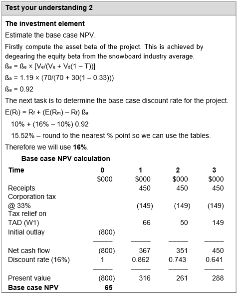
Test your understanding 2
Rounding plc is a company currently engaged in the manufacture of baby equipment. It wishes to diversify into the manufacture of snowboards.
The investment details
The company’s equity beta is 1.27 and is current debt to equity ratio is 25:75, however the company’s gearing ratio will change as a result of the new project.
Firms involved in snowboard manufacture have an average equity beta of 1.19 and an average debt to equity ratio of 30:70.
Assume that the debt is risk free, that the risk free rate is 10% and that the expected return from the market portfolio is 16%.
The new project will involve the purchase of new machinery for a cost of $800,000 (net of issue costs), which will produce annual cash inflows of $450,000 for 3 years. At the end of this time it will have no scrap value.
Corporation tax is payable in the same year at a rate of 33%. The machine will attract tax allowable depreciation of 25% pa on a reducing balance basis, with a balancing allowance at the end of the project life when the machine is scrapped.
| The financing details: | |
| The new investment will be financed as follows: | |
| Bonds (redeemable in three years’ time): | 40% |
| Rights issue of equity: | 60% |
The issue costs are 4% on the gross equity issued and 2% on the gross debt issued. Assume that the debt issue costs are tax deductible.
Required:
Calculate the adjusted present value of the project.
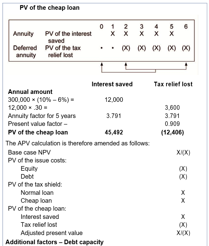
Additional factors regarding the APV method Additional factors – Subsidised/cheap loans
If a loan is cheap, the interest cost is lower. However, the benefit is reduced since the tax shield will also be lower:
| PV of the cheap loan (opportunity benefit): | |
| PV of the interest saved | X |
| Less: PV of the tax relief lost | (X) |
| PV of the cheap loan | ––– |
| X | |
| ––– |
Example: A plc requires $1 million in debt finance for 5 years.
It has borrowed $700,000 in the form of 10% bonds redeemable in
5 years and the remainder under a government subsidised loan scheme at 6%. The tax rate is 30%. Assume that tax is delayed one year.
Calculate the PV of the tax shields and the PV of the cheap loan.
- PV of the tax shields
Although the cheap loan has a cost of 6% it has the same risk as a normal loan, therefore the appropriate discount rate is 10% pa.
| Annual tax relief = Total loan × | Normal loan | Cheap loan |
| interest rate × tax rate | ||
| 700,000 × 0.10 × .30 = | 21,000 | 5,400 |
| 300,000 × 0.06 × .30 = | ||
| Annuity factor for 5 years @10% | 3.791 | 3.791 |
| Discount factor for 1 year @10% | 0.909 | 0.909 |
| PV of the tax shield | 72,366 | 18,609 |
Debt finance benefits a project because of the associated tax shield. If a project brings about an increase in the borrowing capacity of the firm, it will increase the potential tax shield available.
An occasional exam trick is to give both the amount of debt actually raised and the increase in debt capacity brought about by the project. It is this theoretical debt capacity on which the tax shield should be based.
A project’s debt capacity denotes its ability to act as security for a loan. It is the tax relief available on such a loan, which gives debt capacity its value.
When calculating the present value of the tax shield (tax relief on interest) it should be based on the project’s theoretical debt capacity and not on the actual amount of the debt used.
The tax benefit from a project accrues from each pound of debt finance that it can support, even if the debt is used on some other project. We therefore use the theoretical debt capacity to match the tax benefit to the specific project.
For example, if a question stated that actual debt raised is $800,000 but you are told in the question ‘The investment is believed to add $1 million to the company’s debt capacity.’ The present value of the tax shield is based on the £1 million – the theoretical amount.
Test your understanding 3
Blades Co is considering diversifying its operations away from its main area of business (food manufacturing) into the plastics business. It wishes to evaluate an investment project, which involves the purchase of a moulding machine that costs $450,000. The project is expected to produce net annual operating cash flows of $220,000 for each of the three years of its life. At the end of this time its scrap value will be zero.
The assets of the project can support debt finance of 40% of its initial cost (including issue costs). Blades is considering borrowing this amount from two different sources.
First, a local government organisation has offered to lend $90,000, with no issue costs, at a subsidised interest rate of 3% per annum. The full $90,000 would be repayable after 3 years.
The rest of the debt would be provided by the bank, at Blades’ normal interest rate. This bank loan would be repaid in three equal annual instalments.
The balance of finance will be provided by a placing of new equity.
Issue costs will be 5% of funds raised for the equity placing and 2% for the bank loan. Debt issue costs are allowable for corporation tax.
The plastics industry has an average equity beta of 1.368 and an average debt:equity ratio of 1:5 at market values. Blades’ current equity beta is 1.8 and 20% of its long-term capital is represented by debt which is generally regarded to be risk free.
The risk free rate is 10% pa and the expected return on an average market portfolio is 15%.
Corporation tax is at a rate of 30%, payable in the same year. The machine will attract a 70% initial tax allowable depreciation allowance and the balance is to be written off evenly over the remainder of the asset life and is allowable against tax. The firm is certain that it will earn sufficient profits against which to offset these allowances.
Required:
Calculate the adjusted present value and determine whether the project is worthwhile.
Advantages and disadvantages of APV
The APV technique has practical advantages and theoretical disadvantages.
Advantages
- Step-by-step approach gives clear understanding of the elements of the decision
Disadvantages
- Based on M&M’s with-tax theory. Therefore ignores:
– Bankruptcy risk
– Tax exhaustion
– Agency costs
Can evaluate any type of
Based on M&M’s with-tax theory.
financing package
Therefore assumes:
– Debt is risk free and
irredeemable
- More straightforward than adjusting the WACC which can be very complex
International CAPM and APV
A recap of the basics
The APV method of investment appraisal has been introduced in this chapter in the context of domestic investments. There are essentially three steps to the technique:
Step 1: Estimate the base case NPV assuming that the project is financed entirely by equity.
Step 2: Estimate the financial ‘side effects’ of the actual method of financing.
Step 3: Add the values from steps 1 and 2 to give the APV.
If the APV is positive, accept the project.
We now examine the applicability of the method in appraising international investments.
Mechanics of the International APV method
The normal procedure of determining the relevant cash flows and discounting at a rate of return commensurate with the project’s risk should be followed as before, but taking account of the international factors as discussed earlier.
The steps therefore become:
Step 1: The base case NPV assumes that the project is financed entirely by equity, so the discount rate must be the cost of equity allowing for the project risk but excluding financial risk – using the international CAPM equation with an ungeared ‘world’ β (see below).
Step 2: Adjustments should be made for
- tax relief on debt interest and issue costs
- subsidies from foreign governments
- projects financed by loans raised locally
- restriction on remittances.
Step 3: Add the values from steps 1 and 2 to give the APV.
This is basically the same approach as for domestic appraisal, with a little more care needed in identifying the appropriate appraisal rates and adjustments.
International CAPM
In the domestic context you should recall that the CAPM could be used to derive the return required as
Rj = Rf + β(Rm – Rf)
where Rj is the required return from the investment Rf is the risk free rate of return
Rm is the expected return from the whole market
- is a measure of the systematic risk of the investment However, where a company operates
- internationally
- in integrated markets.
investors should therefore consider applying the international cost of capital to investment appraisal, rather than a domestic CAPM.
The logic:
- A company involved in international operations, will, in addition to the usual risk, be exposed to:
– currency risk
– political risk.
These are mainly unsystematic and can be diversified away by holding an internationally diversified portfolio.
- For example, a fully diversified UK investor can achieve further risk reduction by investing in other countries. Part of the systematic risk of the UK market is in fact unsystematic risk from an international viewpoint.
The international CAPM equation will therefore read:
Rj = Rf + βw (Rw – Rf)
where
Rj is the required return
Rw is the expected return from the whole world portfolio
βw is a measure of the project’s world systematic risk, i.e. how returns on the investment correlate with those on the world market.
In the UK, for example, the return from the whole market could be estimated from looking at domestic stock market indexes such as the FTSE All-Share index, which covers about 600 of the top shares listed in the UK.
This basic CAPM model is valid for:
- a company or investor with domestic investments only, or
- investments in a country with segmented markets, as opposed to integrated markets.
Integrated capital markets exist if investors can invest in any country that does not impose restrictions on capital movements. Segmented markets are associated with a closed economy, or markets where switching investments from country to country is not easily achieved, such as in many service industries.
It is argued that:
- Investors can diversify their risk more effectively in an integrated market, because more investments are available and returns on domestic and foreign assets are not perfectly correlated.
- The cost of capital is lower if markets are integrated than in a closed economy. Companies whose shareholders are international investors should therefore consider applying the international cost of capital to investment appraisal, rather than a domestic CAPM.
This can be done by looking at the international CAPM.
In practice it is impossible to hold a share of the whole world portfolio, but significant international diversification can be achieved by:
- direct holdings in overseas companies
- holdings in unit trusts specialising in overseas companies
- investing in multinational companies.
You should appreciate that in principle risk reduction can be achieved either by investing directly in an international portfolio of shares or investing in local companies with significant overseas activities.
Implications of the international capital asset pricing model (or IAPM) are that:
- When setting a cost of capital, a company should assess the nature of its investors and their investment portfolios.
- If markets are segmented, investments that are profitable for an international/foreign company might not be profitable for a domestic company, because the international company will have a lower cost of capital.
However, the validity of the international capital asset pricing model rests on the assumption that capital markets are fully integrated and investors are ‘world’ investors. In practice, this is not necessarily the case.
Countries and capital markets are not fully integrated, since there are costs to foreign investment and domestic investors often have better access to information than foreign investors.
In conclusion, although the international capital asset pricing model can in theory be applied, there remain valid reasons for measuring the cost of equity on the basis of a domestic market portfolio and the basic CAPM.
| (3) The APV calculation | |||
| Base cost NPV | 65,000 | ||
| Less: PV of issue costs: | |||
| Equity | (20,000) | ||
| Debt | (4,376) | ||
| Plus PV of tax shield | 26,800 | ||
| ––––––– | |||
| Therefore adjusted present value is | $67,424 | ||
| ––––––– | |||
Based upon these estimates the project appears financially viable.
Test your understanding 3
Step 1: Base case net present value
First compute the ungeared (asset) beta for this project type (based on the equity beta for the plastics industry).
| ßa = ße × | Ve | |||||
| Ve+ Vd (1–T) | ||||||
| = 1.368 × [5/(5 + 1(1 – 0.30))] | ||||||
| = 1.2 | ||||||
| Required return of project | = 10% + (15% –10%) 1.2 | |||||
| = 16% pa. | ||||||
| Then discount the project cash flows at 16% | ||||||
| Time | 0 | 1 | 2 | 3 | ||
| $000 | $000 | $000 | $000 | |||
| Equipment | (450) | |||||
| TAD (W1) | 94.5 | 20.25 | 20.25 | |||
| Operating cash flows | 220.00 | 220.00 | 220.00 | |||
| Tax on operating cash flows | (66.00) | (66.00) | (66.00) | |||
| ——— | ——— | ——— | ——— | |||
| (450) | 248.5 | 174.25 | 174.25 | |||
| ——— | ——— | ——— | ——— | |||
| 16% factors | 1 | 0.862 | 0.743 | 0.641 | ||
| PV | (450) | 214.21 | 129.47 | 111.69 | ||
| Base case NPV = | $5,370 | |||||
| Workings | ||
| (W1) – Tax allowable depreciation | ||
| Tax @ 30% | ||
| $ | $ | |
| Cost of machine | 450,000 | |
| First year allowance (70%) | 315,000 | 94,500 |
| ––––––– | ||
| 135,000 | ||
| TAD allowances (straight line) | ––––––– | |
| (for each of next two years) | 67,500 | 20,250 |
Step 2: Adjusted present value (the financing side effects)
| Lay out the financing package: | |
| Capital requirements: | $ |
| Equity (60%) | 270,000 |
| Subsidised debt | 90,000 |
| Bank loan | 90,000 |
| ––––––– | |
| 450,000 | |
| ––––––– | |
| $ | |
| Issue costs: | |
| (i) Equity 5/95 × 270,000 | 14,210 |
| (ii) Debt 2/98 × 90,000 | 1,837 |
| Issue costs on debt at T0 | ($1,837) |
| Tax relief at 30% | $551 |
| ––––––– | |
| PV of the issue costs on debt | ($1,286) |
- Tax relief on loan interest
Gross value of bank loan = $90,000 + $1,837 (issue costs) = $91,837
Annual repayments = $91,837/2.487 = $36,927
| Loan schedule | ||||||
| Year | Opening | Interest | Repayment | Closing | ||
| balance | $ | balance | ||||
| $ | $ | $ | ||||
| 1 | 91,837 | 9,184 | 36,927 | 64,094 | ||
| 2 | 64,094 | 6,409 | 36,927 | 33,576 | ||
| 3 | 33,576 | 3,358 | 36,927 | 7 (rounding | ||
| diff) | ||||||
Subsidised loan interest will be 3% of $90,000 each year for 3 years, i.e. $2,700 per annum.
Tax relief at 30% on interest:
| Year | Cash | 10% factor | PV |
| $ | $ | ||
| 1 | 30% × | ||
| (9,184 + 2,700) | 0.909 | 3,241 | |
| 2 | 30% × | ||
| (6,409 + 2,700) | 0.826 | 2,257 | |
| 3 | 30% × | ||
| (3,358 + 2,700) | 0.751 | 1,365 | |
| ––––– | |||
| 6,863 | |||
| ––––– |
- Interest saving on subsidised loan
Saving = $90,000 × (10% – 3%) = $6,300 per annum
Present value of saving (post-tax) = $6,300 × (1 – 0.30) × 2.487 = $10,968
| Step 3: Adjusted present value | |
| $ | |
| Base case NPV | 5,370 |
| Issue costs – equity | (14,210) |
| Issue costs – debt | (1,286) |
| Tax shield | 6,863 |
| Value of subsidy | 10,968 |
| –––––– | |
| The project APV is | 7,705 |
| –––––– |
The project will increase shareholder wealth by $7,705, so the project funded in this way is acceptable.