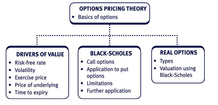
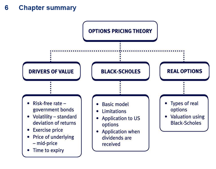
The principles of option pricing theory
Option terminology An option
The right but not an obligation, to buy or sell a particular good at an exercise price, at or before a specified date.
Call option
The right but not an obligation to buy a particular good at an exercise price.
Put option
The right but not an obligation to sell a particular good at an exercise price.
Exercise/strike price
The fixed price at which the good may be bought or sold.
American option
An option that can be exercised on any day up until its expiry date.
European option
An option that can only be exercised on the last day of the option.
Premium
The cost of an option.
Traded option
Standardised option contracts sold on a futures exchange (normally American options).
Over the counter (OTC) option
Tailor-made option – usually sold by a bank (normally European options).
Option value
The key aspect to an option’s value is that the buyer has a choice whether or not to use it. Thus the option can be used to avoid downside risk exposure without foregoing upside exposure.
The value of an option is made up of two components. These are illustrated below for a call option:
The intrinsic value
The intrinsic value looks at the exercise price compared with the price of the underlying asset.
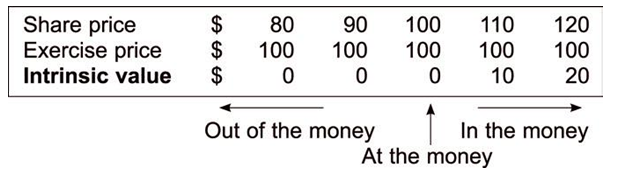
- The value of the call option will increase as the share price increases. Conversely a lower exercise price would also give a higher option value.
- An option can never have a negative intrinsic value. If the option is out of the money, then the intrinsic value is zero.
- On the expiry date, the value of an option is equal to its intrinsic value.
The time value
- Time to expiry.
– As the period to expiry increases, the chance of a profit before the expiry date grows, increasing the option value.
- Volatility of the share price.
– The holder of a call option does not suffer if the share price falls below the exercise price, i.e. there is a limit to the downside.
– However the option holder gains if the share price increases above the exercise price, i.e. there is no limit to the upside.
– Thus the greater the volatility the better, as this increases the probability of a valuable increase in share price.
- Risk-free interest rate.
– As stated above, the exercise price has to be paid in the future, therefore the higher the interest rates the lower the present value of the exercise price. This reduces the cost of exercising and thus adds value to the current call option value.
– Alternatively, since having a call option means that the share purchase can be deferred, owning a call option becomes more valuable when interest rates are high, since the money left in the bank will be generating a higher return.
Summary of the determinants of call option prices:
Increase in
Value of a call
Share price
Increase
Exercise price
Decrease
Time to expiry
Increase
Volatility (s)
Increase
Interest rate
Increase
Test your understanding 1
Complete the following table for put options.
Summary of the determinants of call option prices:
| Increase in | Call | Put |
| Share price | Increase | |
| Exercise price | Decrease | |
| Time to expiry | Increase | |
| Volatility – s | Increase | |
| Interest rate | Increase |
Test your understanding 2
A pension fund manager is concerned that the value of the stock market will fall.
Required:
Suggest an option strategy he could use to protect the fund value.
The drivers of option value in practice – Introduction
As discussed above, the main drivers of option value are as follows:
- value of the underlying asset
- exercise price
- time to expiry
- volatility
- risk-free rate.
Determining these figures in practice is discussed below:
Value of the underlying asset
- For quoted underlying assets a value can be looked up on the market. Most markets give prices for buying and selling the underlying asset. A mid-price is usually used for option pricing.
For example, if a price is quoted as 243–244 cents, then a mid-price of 243.5 cents should be used.
- In the case of unquoted underlying assets a separate exercise must be undertaken to value them.
For example, suppose an unquoted company has issued share options to employees as part of their remuneration package. To value these call options (e.g. for disclosure or taxation purposes) one must first value the shares using, e.g. P/E ratios.
Exercise price and time to expiry
Both the exercise price and expiry date are stated in the terms of the option contract.
Volatility
- Volatility represents the standard deviation of day-to-day price changes in a security, expressed as an annualised percentage. Two measures of volatility are commonly used in options trading: historical and implied.
- Historical volatility can be measured by observing price changes of a security over a period of time. It is not necessarily a forecast of future volatility, but can be used to determine the option price.
- Implied volatility can be calculated by taking current quoted options prices and working backwards.
A common approach to calculating historical volatility is as follows:
- Calculate the daily return using (current price/previous day’s price) or Pn/Pn–1.
- Take the log of each ‘return’ to convert into a continuous return.
- Calculate the standard deviation of the logs to get a daily volatility.
- Annualise the result.
| Volatility calculation | ||||||
| Day | Price | Pn/Pn–1 | ln(Pn/Pn–1) | |||
| ‘x’ | x2 | |||||
| Monday | 100 | |||||
| Tuesday | 101 | 1.010000 | 0.009950 | 0.000099 | ||
| Wednesday | 105 | 1.039604 | 0.038840 | 0.001509 | ||
| Thursday | 103 | 0.980952 | –0.019231 | 0.000370 | ||
| Friday | 104 | 1.009709 | 0.009662 | 0.000093 | ||
| Sum | 0.039221 | 0.002071 | ||||
| Average | 0.009805 | 0.000518 | ||||
In order to calculate the volatility (standard deviation) we need to use these two final figures.
Volatility = square root of (the average value of x2 less the square of the average value of x)
- √ (0.000518 – 0.0098052)
- 0205 or approximately 2%
Assuming 260 trading days on the market, Annualised volatility = daily volatility × √260 = 0.33 or 33%.
The method for calculating the continuous return in the above example may be unfamiliar to you. The basic idea is that instead of dividing a time period into years or weeks or days for discounting purposes we can discount continuously. To get the same answer either way, we need to set continuous rate = ln (1 + discrete rate)
For example, if the discrete rate is 10% p.a., then a continuous rate is given by:
Continuous rate = ln 1.10 = 0.0953 or 9.53%.
Discount factors using continuous rates are given by DF = e– it where i is the continuous rate and t the time period.
Risk-free rate
- The risk-free rate is the minimum return required by investors from a risk-free investment.
- Treasury bills or other short-term (usually three months). Government borrowings are regarded as the safest possible investment and their rate of return is often given in a question to be used as a figure for the risk-free rate.
The Black-Scholes option pricing model
Introduction
The Black -Scholes model values call options before the expiry date and takes account of all five factors that determine the value of an option.
Using the Black-Scholes model to value call options
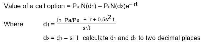
Note: The formula is daunting, but fortunately you do not need to learn it, as it will be given in the examination paper. You need to be aware only of the variables which it includes, to be able to plug in the numbers.
The key:
Pa = current price of underlying asset (e.g. share price)
Pe = exercise price
r = risk-free rate of interest
t = time until expiry of option in years
s = volatility of the share price (as measured by the standard deviation expressed as a decimal)
N(d) = equals the area under the normal curve up to d (see normal distribution tables)
e = 2.71828, the exponential constant
In = the natural logarithm (logarithm base ‘e’)
Pee–rt = present value of the exercise price calculated by using continuous discounting factors.
Measures of volatility
Standard deviation and variance
The measure of volatility used in the Black-Scholes model is the annual standard deviation (s), expressed as a decimal.
Past exam questions have occasionally quoted volatility in terms of the ‘variance’, which is the square of the standard deviation. In this case, take the square root of the given variance figure to give the volatility in the correct terms for the Black-Scholes formula.
Alternatively, monthly, or weekly, standard deviations may be quoted. To convert from a monthly standard deviation to an annual figure
- square the monthly standard deviation
- multiply by 12
- take the square root of the result.
This will now be the annual standard deviation figure as required.
Normal distribution tables
Recap of normal distributions
Extract from standard normal distribution table
| 0.00 | 0.01 | 0.02 | 0.03 | 0.04 | 0.05 | 0.06 | 0.07 | 0.08 | 0.09 | |
| 0.0 | .0000 | .0040 | .0080 | .0120 | .0159 | .0199 | .0239 | .0279 | .0319 | .0359 |
| 0.1 | .0398 | .0438 | .0478 | .0517 | .0557 | .0596 | .0636 | .0675 | .0714 | .0753 |
| 0.2 | .0793 | .0832 | .0871 | .0910 | .0948 | .0987 | .1026 | .1064 | .1103 | .1141 |
| 0.3 | .1179 | .1217 | .1255 | .1293 | .1331 | .1368 | .1406 | .1443 | .1480 | .1517 |
| 0.4 | .1554 | .1591 | .1628 | .1664 | .1700 | .1736 | .1772 | .1808 | .1844 | .1879 |
| 0.5 | .1915 | .1950 | .1985 | .2019 | .2054 | .2088 | .2123 | .2157 | .2190 | .2224 |
| 0.6 | .2257 | .2291 | .2324 | .2357 | .2389 | .2422 | .2454 | .2486 | .2518 | .2549 |
| 0.7 | .2580 | .2611 | .2642 | .2673 | .2704 | .2734 | .2764 | .2794 | .2823 | .2852 |
| 0.8 | .2881 | .2910 | .2939 | .2967 | .2995 | .3023 | .3051 | .3078 | .3106 | .3133 |
| 0.9 | .3159 | .3186 | .3212 | .3238 | .3264 | .3289 | .3315 | .3340 | .3365 | .3389 |
| 1.0 | .3413 | .3438 | .3461 | .3485 | .3508 | .3531 | .3554 | .3577 | .3599 | .3621 |
| 1.1 | .3643 | .3665 | .3686 | .3708 | .3729 | .3749 | .3770 | .3790 | .3810 | .3830 |
| 1.2 | .3849 | .3869 | .3888 | .3907 | .3925 | .3944 | .3962 | .3980 | .3997 | .4015 |
| 1.3 | .4032 | .4049 | .4066 | .4082 | .4099 | .4115 | .4131 | .4147 | .4162 | .4177 |
| 1.4 | .4192 | .4207 | .4222 | .4236 | .4251 | .4265 | .4279 | .4292 | .4306 | .4319 |
| 1.5 | .4332 | .4345 | .4357 | .4370 | .4382 | .4394 | .4406 | .4418 | .4430 | .4441 |
| 1.6 | .4452 | .4463 | .4474 | .4485 | .4495 | .4505 | .4515 | .4525 | .4535 | .4545 |
| 1.7 | .4554 | .4564 | .4573 | .4582 | .4591 | .4599 | .4608 | .4616 | .4625 | .4633 |
| 1.8 | .4641 | .4649 | .4656 | .4664 | .4671 | .4678 | .4686 | .4693 | .4699 | .4706 |
| 1.9 | .4713 | .4719 | .4726 | .4732 | .4738 | .4744 | .4750 | .4756 | .4762 | .4767 |
This table can be used to calculate N(d1), the cumulative normal distribution function needed for the Black-Scholes model of option pricing.
- If d1 > 0, add 0.5 to the relevant number above.
- If d1 < 0, subtract the relevant number above from 0.5. For example if d1 is 1.05, N(d1) = 0.3531 + 0.5 = 0.8531.
Note: N(d) = Is the area under the normal curve up to d in the shaped area of the figure below.
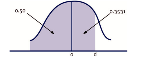
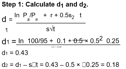
Illustration of the Black-Scholes model
| The current share price of B plc shares | = | $100 | ||
| The exercise price | = | $95 | ||
| The risk-free rate of interest | = | 10% pa | = | 0.1 |
| The standard deviation of return on the | ||||
| shares | = | 50% | = | 0.5 |
| The time to expiry | = | 3 months | = | 0.25 |
Required:
Calculate the value of the above call option.
Solution
Step 2: Use normal distribution tables to find the value of N(d1) and N(d2).
N(d1) = 0.5 + 0.1664 = 0.6664
N(d2) = 0.5 + 0.0714 = 0.5714
Step 3: Plug these numbers into the Black-Scholes formula.
Value of a call option = Pa N(d1) – PeN(d2)e–rt
- 100 × 0.6664 – 95 × 0.5714 × e–(0.1 × 0.25)
- $13.70
Note: This can be split between the intrinsic value of $5 (100 – 95) and the time value which is $8.70.
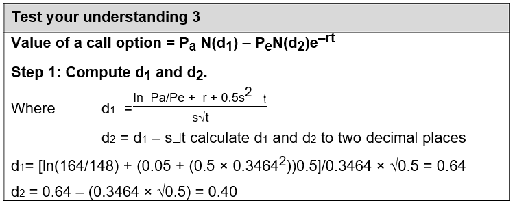
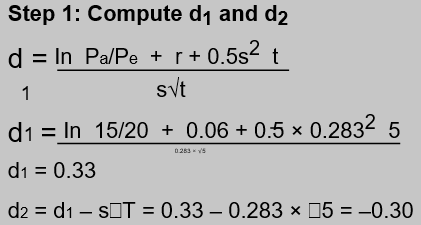
Test your understanding 3
Suppose that the risk-free rate is 5% and the standard deviation of the return on the share in the past has been estimated as 34.64%.
Required:
Estimate the value of a six-month call option at an exercise price of $1.48 (current share price = $1.64).
Using the Black-Scholes model to value put options
If you have calculated the value of a call option using Black -Scholes, then the value of a corresponding put option can be found using the put call parity formula.
The put call parity equation is on the examination formula sheet:
Put call parity P= c – Pa + Pe × e–rt
Step 1: Value the corresponding call option using the Black-Scholes model.
Step 2: Then calculate the value the put option using the put call parity equation.
Black-Scholes model: value put options
Returning to the earlier example of B plc, where the current share price is $100, exercise price is $95, the risk -free rate of interest is 10%, the standard deviation of shares return is 50% and the time to expiry is three months, calculate the value of a put option.
Solution
- Step 1: We have already calculated the value of the call option at $13.70.
- Step 2: Using put call parity equation:
Put call parity P= c – Pa + Pe × e–rt
Value of a put = 13.70 – 100.00 + 92.65
= $6.35
Test your understanding 4
Using the information given in TYU3, calculate the value of the corresponding put option.
Underlying assumptions and limitations
The model assumes that:
- The options are European calls.
- There are no transaction costs or taxes.
- The investor can borrow at the risk-free rate.
- The risk-free rate of interest and the share’s volatility is constant over the life of the option.
- The future share-price volatility can be estimated by observing past share price volatility.
- The share price follows a random walk and that the possible share prices are based on a normal distribution.
- No dividends are payable before the option expiry date.
In practice these unrealistic assumptions can be relaxed and the basic model can be developed to reflect a more complex situation.
Delta and delta hedges
The figure N(d1) is known as delta. Delta measures the change in option value which would result from a $1 change in the value of the underlying asset (e.g. share).
An investor can eliminate the risk of his shareholding by constructing a ‘delta hedge’.
- An investor who holds a number of shares and sells (an option writer) a number of call options in the proportion dictated by the delta (the hedge ratio) ensures a hedged portfolio. B. A hedged portfolio is one where the gains and losses cancel out against each other.
- Number of option calls to sell = Number of shares held/N(d1).
- Alternatively, if you have already written call options, then a delta hedge can be constructed by buying shares.
- Number of shares to hold = Number of call options sold × N(d1).
Because share prices change continuously in the real world, the value of delta also changes continuously. Therefore, the investor who wants to maintain a risk neutral position will have to continuously adjust the balance of options and shares in his portfolio. This process is known as ‘dynamic delta hedging’.
Example of a delta hedge
Assuming a call option currently has a delta of 0.5, let use it to construct a hedged portfolio for an investor who holds 100 shares.
The investor in shares will find out how many call options he will have to (write) sell.
So if you had 100 shares we would need to sell (100 shares/0.5) = 200 calls to construct a delta hedge. The number of options will exceed the number of shares unless the delta is 1, then they would be an equal number of each.
The call option writers (the seller of the call options) will find out how many shares they will have to buy.
If the share price increases by 10 cents, the call options increase by
5 cents. However as we have sold the call option our portfolio decreases by 5 cents for every call option sold.
| The Comfort | Delta | Number of | Number of | Overall gain |
| Table: | shares | call options | or loss is | |
| purchased | sold | zero. | ||
| Delta neutral | ||||
| Current position | 0.5 | 100 | 200 | |
| Share price | $10 | (–5c × 200) | 0 | |
| increases by 10c | –$10= |
However, the difficulty is that the delta value is not at a constant. It changes as the share price changes.
Suppose that the 10 cents move in the share price caused the delta to move to 0.7. The option writer will need to buy 200 calls × 0.7 = 140 shares in order to hedge the position, i.e. 40 extra shares.
The portfolio will need rebalancing as the delta value changes. The frequency of this depends on the rate of change of delta, measured by gamma.
Gamma, vega, rho and theta
Delta measures the sensitivity of the option value to changes in the value of the underlying asset (explained in detail above).
Sensitivities to other factors in the Black Scholes formula are denoted by other Greek letters as follows:
Gamma – measures the rate of change of delta as the underlying asset’s price changes.
Vega – measures the sensitivity of an option’s value to a change in the implied volatility of the underlying asset.
Rho – measures the sensitivity of the option value to changes in the risk free rate of interest.
Theta – measures the rate of decline in the value of the option caused by the passage of time.
More details on ‘The Greeks’
Collectively, delta, gamma, vega, rho and theta are known as ‘The Greeks’.
The importance of the delta value has been illustrated above i.e. it is useful when setting up a delta hedge. The importance of the other Greeks is explained below.
Gamma
A high gamma value indicates that the delta value is quite volatile.
This means that it will be quite difficult for an option writer to maintain a delta hedge, since the volatile delta value will require the option writer to be constantly changing the number of options written.
Therefore, gamma is a measure of how easy risk management will be.
Vega
The vega determines the sensitivity of an option’s value to a change in the implied volatility of the underlying asset. Implied volatility is what the market is implying the volatility of the underlying asset will be in the future, based on the price changes in an option. The option price may change independently of whether or not the underlying asset’s value changes, due to new information being presented to the markets. Implied volatility is the result of this independent movement in the option’s value, and this determines the vega.
The vega only impacts the time value of an option and as the vega increases, so will the value of the option.
Rho
Interest rates tend to change slowly and by small amounts, so the impact of interest rates on option prices (measured by rho) is generally not particularly significant.
However, note that rho is positive for call options (an increase in interest rates leads to an increase in option price) but negative for puts (an increase in interest rates leads to a decrease in option price).
Also, longer term options have larger rhos than short term options, because the more time there is until expiry of the option, the more significant a change in interest rates is.
Theta
An option price has two components, the intrinsic value and the time value. However, when the option expires, the time premium reduces to zero. Therefore, theta measures how much value is lost over time.
Theta is usually expressed as an amount lost per day (e.g. theta could be
–$0.06, indicating that 6 cents of value is lost per day. Theta usually increases as the expiry date approaches.
Identifying real options in investment appraisal
Introduction
- Flexibility adds value to an investment.
- Financial options are an example where this flexibility can be valued.
- Conventional investment-appraisal techniques typically undervalue flexibility within projects with high uncertainty.
- Real options theory attempts to classify and value flexibility in general by taking the ideas of financial options pricing and developing them.
More detail on valuing flexibility
- Flexibility adds value to an investment:
– For example, if an investment can be staggered, then future costs can be avoided if the market turns out to be less attractive than originally expected.
– The core to this value lies in reducing downside risk exposure but keeping upside potential open – i.e. in making probability distributions asymmetric.
- Financial options are an example where this flexibility can be valued.
– A call option on a share allows an investor to ‘wait and see’ what happens to a share price before deciding whether to exercise the option and will thus benefit from favourable price movements without being affected by adverse movements.
- Conventional investment-appraisal techniques typically undervalue flexibility within projects with high uncertainty.
– High uncertainty within a NPV context will result in a higher discount rate and a lower NPV. However, with such uncertainty any embedded real options will become more valuable.
- Real options theory attempts to classify and value flexibility in general by taking the ideas of financial options pricing and developing them:
– A financial option gives the owner the right, but not the obligation, to buy or sell a security at a given price. Analogously, companies that make strategic investments have the right, but not the obligation, to exploit these opportunities in the future.
– As with financial options most real options involve spending more up front (analogous to the option premium) to give additional flexibility later.
Different types of real option
There are many different classifications of real options. For the purposes of the
AFM syllabus, we use the following four generic headings:
Options to delay/defer
The key here is to be able to delay investment without losing the opportunity, creating a call option on the future investment.
Illustration 1 – Identifying real options in investment appraisal
For example, establishing a drugs patent allows the owner of the patent to wait and see how market conditions develop before producing the drug, without the potential downside of competitors entering the market.
(Note: Drugs patents was the subject of a past examination question on this area. However, there is some debate whether or not patents are real options. This debate is outside the scope of the syllabus.)
Options to switch/redeploy
It may be possible to switch the use of assets should market conditions change.
Illustration 2 – Identifying real options in investment appraisal
For example, traditional production lines were set up to make one product. Modern flexible manufacturing systems (FMS) allow the product output to be changed to match customer requirements.
Similarly a new plant could be designed with resale and/or other uses in mind, using more general-purpose assets than dedicated to allow easier switching.
Illustration 3 – Identifying real options in investment appraisal
For example, when designing a plant management can choose whether to have higher or lower operating gearing. By having mainly variable costs, it is financially more beneficial if the plant does not have to operate every month.
Options to expand/follow-on
It may be possible to adjust the scale of an investment depending on the market conditions.
Options to abandon
If a project has clearly identifiable stages such that investment can be staggered, then management have to decide whether to abandon or continue at the end of each stage.
Illustration 4 – Identifying real options in investment appraisal
When looking to develop their stadiums, many football clubs face the decision whether to build a one- or a two-tier stand:
- A one-tier stand would be cheaper but would be inadequate if the club’s attendance improved greatly.
- A two-tier stand would allow for much greater fan numbers but would be more expensive and would be seen as a waste of money should attendance not improve greatly.
Some clubs (e.g. West Bromwich Albion in the UK) have solved this problem by building a one-tier stand with stronger foundations and designed in such a way (e.g. positioning of exits, corporate boxes, etc.) that it would be relatively straightforward to add a second tier at a later stage without knocking down the first tier.
Such a stand is more expensive than a conventional one-tier stand but the premium paid makes it easier to expand at a later date when (if!) attendance grows.
Illustration 5 – Identifying real options in investment appraisal
Amazon.com undertook a substantial investment to develop its customer base, brand name and information infrastructure for its core book business.
This in effect created a portfolio of real options to extend its operations into a variety of new businesses such as CDs, DVDs, etc.
Test your understanding 5
Comment on a strategy of vertical integration in the context of real options.
Test your understanding 6
A film studio has three new releases planned for the Christmas period but does not know which will be the biggest hit for allocating marketing resources. It thus decides to do a trial screening of each film in selected cinemas and allocates the marketing budget on the basis of the results.
Required:
Comment on this plan using real option theory.
4 Valuing real options
Introduction
Valuing real options is a complex process and currently a matter of some debate as to the most suitable methodology. Within the AFM syllabus you are expected to be able to apply the Black-Scholes model to real options.
Using the Black-Scholes model to value real options
The Black-Scholes equation is well suited for simple real options, those with a single source of uncertainty and a single decision date. To use the model we need to identify the five key input variables as follows:
Exercise price
For most real options (e.g. option to expand, option to delay), the capital investment required can be substituted for the exercise price. These options are examples of call options.
For an option to abandon, use the salvage value on abandonment. This is an example of a put option.
Value of the underlying asset (share price in the earlier calculations)
The value of the underlying asset is usually taken to be the PV of the future cash flows from the project (i.e. excluding any initial investment).
This could be the value of the project being undertaken for a call option (e.g. option to expand, option to delay), or the value of the cash flows being foregone for a put option (option to abandon).
Time to expiry
This is straightforward if the project involves a single investment.
Volatility
The volatility of the underlying asset (here the future operating cash flows) can be measured using typical industry sector risk.
Risk-free rate
Many writers continue to use the risk-free rate for real options. However, some argue that a higher rate be used to reflect the extra risks when replacing the share price with the PV of future cash flows.
Illustration 6 – Valuing real options
A UK retailer is considering opening a new store in Germany with the following details (note that all figures have been converted into the domestic currency):
| | Estimated cost | | £12m |
| Present value of net receipts | | £10m | |
| | NPV | | –£2m |
These figures would suggest that the investment should be rejected. However, if the first store is opened then the firm would gain the option to open a second store (an option to expand or follow-on).
Suppose this would have the following details:
- Timing (t)
- Estimated cost (Pe)
- Present value of net receipts (Pa)
- Volatility of cash flows (s)
- Risk-free rate (r)
- 5 years’ time
- £20m
- £15m
- 3%
- 6%
The value of the call option on the second store is then calculated as normal using Black-Scholes:
| Step 2: Compute N(d1) and N(d2). | |
| N(d1) = 0.5 + 0.1293 = 0.6293 | |
| N(d2) = 0.5 – 0.1179 = 0.3821 | |
| Step 3: Use formula. | |
| Value of a call option | = Pa N(d1) –PeN(d2)e–rt |
| = 15 × 0.6293 – 20 × 0.3821 × e–(0.06 × 5) | |
| = £3.8m | |
| Summary | |
| £m | |
| Conventional NPV of first store | (2) |
| Value of call option on second store | 3.8 |
| ––– | |
| Strategic NPV | 1.8 |
| ––– | |
| The project should thus be accepted. |
Test your understanding 7
An online DVD and CD retailer is considering investing $2m on improving its customer information and online ordering systems. The expectation is that this will enable the company to expand by extending its range of products. A decision will be made on the expansion in 1 year’s time, when the directors have had chance to analyse customer behaviour and competitors’ businesses in more detail, to assess whether the expansion is worthwhile.
Preliminary estimates of the expansion programme have found that an investment of $5m in 1 year’s time will generate net receipts with a present value of $4m in the years thereafter. The project’s cash flows are expected to be quite volatile, with a standard deviation of 40%.
The current risk free rate of interest is 5%.
Required:
Advise the firm whether the initial investment in updating the systems is worthwhile.
Further numerical example – Option to abandon
The real options considered in the above examples were call options (i.e. there was an option to buy into a project). All options to delay/defer, options to switch/redeploy and options to expand/follow-on are call options.
By contrast, an option to abandon is a put option, in that now the business has an option to sell the assets used in the project.
Numerical example
ABC Co is considering investing in the following project:
| $000 | T0 | T1 | T2 | T3 | T4 |
| PV of cash flows | (100) | 12 | 15 | 30 | 35 |
So the NPV of the project is negative (–$8,000) and the project would be rejected.
However, if the company had the option to abandon the project after 2 years (i.e. at T2) and to receive $ 70,000 for the sale of the assets, consider the value of this option to abandon, and the impact on the decision. (Assume that the risk free rate is 5% and that the volatility associated with the project cash flows is 20%).
It is critical that we can correctly identify the five variables to input into the Black-Scholes model.
For the option to abandon, these are as follows:
Pa = PV of cash flows foregone if we abandon = $30,000 + $35,000 = $65,000
s = standard deviation of the project cash flows = 20% Pe = abandonment proceeds = $70,000
t = time until abandonment = 2 years
r = risk free interest rate = 5%
Calculate Black Scholes figures
d1 = 0.23
d2 = –0.05
N(d1) = 0.5910
N(d2) = 0.4801
Calculating the main formula gives a call option value of $8,006
Therefore, using put-call parity, the put option value is $6,342
In this case the project, even when considering the possibility of abandonment after two years, is still not acceptable.
It has a strategic NPV of –$8,000 (basic NPV) + $6,342 (value of real option) = –$1,658.
Using real options when making financial strategy decisions
Manics Co is considering investing in the following project:
| $m | T0 | T1 | T2 | T3-T8 |
| Free cash flows | (500) | 120 | (200) | 160 |
At a discount rate of 10%, the NPV of the project is positive (approximately $19.7m NPV).
This is a very small positive NPV, so some of the directors have expressed concerns about the sensitivity of the project to possible changes in the forecast cash flows.
However, the financial manager feels that the project is being unfairly under-valued, so he has prepared some further analysis of the project.
The key to the financial manager’s concern is that he feels that the large cash outflow at the end of year 2 is discretionary and does not have to be made (in particular if circumstances have changed and the project is not proving to be as successful as had been hoped).
He has therefore split the original project into two: an initial investment of $500m which will produce net cash inflows of $120m for the following
8 years, and a further investment of $320m after two years which will increase the net cash inflows by $40m to $160m per year for the remaining six years.
The project is now being viewed as an initial expansion costing $500m – phase 1 – followed by an option to expand further after two years – phase 2.
If separate NPV calculations are carried out for each of these phases (again using 10% as the discount rate), the results below are obtained:
Phase 1: NPV = $140.2m positive
Phase 2: NPV = $120.5 negative
Note that the overall NPV is $140.2m – $120.5m = $19.7m as before.
This extra analysis provides some interesting insight. Given that there is no obligation for the company to carry out phase 2, the overall NPV must be at least $140.2m, which far exceeds the initial NPV calculated of $19.7m.
Although phase 2 does not currently seem worthwhile, the option to carry out this phase can only add value as an option can never have a negative value.
If the cash flows expected from phase 2 were to become favourable, the company will have the ability to carry out phase 2 and reap the benefit.
Hence, the overall NPV will be $140.2m plus the value of the option to carry out phase 2.
The financial manager has therefore used the BSOP model to value the option to expand (real option), as shown below.
The inputs required for the Black Scholes option pricing (BSOP) formula are:
Pe = the investment required after two years to carry out phase 2 = $320m
Pa = the PV of the net cash inflows currently forecast to arise from phase two = $144.0m (this must exclude the Pe)
t = the time until phase 2 will begin = 2 years
The s and r figures (volatility and risk free rate respectively) have not been presented yet in this example, but they will both be given within any exam question.
Assume that s is 50% and r is 5% here.
Using these inputs the option value can now be calculated:
d1 = –0.63
d2 = –1.34
N(d1) = 0.2643
N(d2) = 0.0901
Value of the call option = $12.0m
Hence, the total NPV for the project with the option to expand
= $140.2m + $12.0m = $152.2m
As a result of the financial manager’s further analysis, a project which initially seemed fairly marginal has been shown to be extremely attractive.
The directors who were expressing concerns about the sensitivity associated with the project will presumably be much happier now to proceed with the project.
The attractiveness of the project arises because phase 1 of the project is itself attractive and the company can potentially benefit if the phase 2 expansion finally becomes worthwhile.
Student Accountant article
The articles ‘Investment appraisal and real options’ and ‘Using real options when making financial strategy decisions’ in the Technical Articles section of the ACCA website provide further details on real options, including some good examples of calculations.
5 Other uses of the Black-Scholes model
Use of the Black-Scholes model in equity valuation
The model can also be used to value the equity of a company.
The basic idea is that, because of limited liability, shareholders can walk away from a company when the debt exceeds the asset value. However, when the assets exceed the debts, those shareholders will keep running the business, in order to collect the surplus.
Therefore, the value of shares can be seen as a call option owned by shareholders – we can use Black-Scholes to value such an option.
Five factors to input into the Black-Scholes model
It is critical that we can correctly identify the five variables to input into the Black-Scholes model.
For equity valuation, these are as follows:
Pa = fair value of the firm’s assets
s = standard deviation of the assets’ value
Pe = amount owed to bank (see below for more details)
t = time until debt is redeemed
r = risk free interest rate
Note that the value of Pe will not just be the redemption value of the debt. The amount owed to the bank incorporates all the interest payments as well as the ultimate capital repayment.
In fact, the value of Pe to input into the Black-Scholes model should be calculated as the theoretical redemption value of an equivalent zero coupon debt.
Deriving Pe
A company has $100 of debt in issue carrying 5% interest and with five years to maturity. The company’s current (pre-tax) cost of debt capital is 8%.
Required:
Calculate the theoretical redemption value of an equivalent zero coupon debt.
| Solution | |||
| Year | Cash flow ($) | DF (8%) | PV |
| 1 | 5 | 0.926 | 4.63 |
| 2 | 5 | 0.857 | 4.29 |
| 3 | 5 | 0.794 | 3.97 |
| 4 | 5 | 0.735 | 3.68 |
| 5 | 105 | 0.681 | 71.51 |
| ––––– | |||
| 88.08 | |||
| ––––– |
The repayment value on a zero coupon bond of the same current market value is calculated by finding the unknown future value which, when discounted at 8% over five years, gives a present value of $88.08.
i.e. 88.08 = Value/1.085
Value = $129.42
Numerical example of BSOP and equity valuation
Sparks is a company in the electronics industry and is looking to expand through acquisition.
A target company, EBMS, has been identified and the directors of Sparks are looking to value the entire equity capital of EBMS.
From discussions with the directors of EBMS, the assets of EBMS have been valued at $1,450m which the directors of EBMS consider to be their fair value in use in the business. The volatility of the asset value has been agreed at 10% per annum.
EBMS currently has 4% bonds in issue with a book value of $900m which are redeemable in 3 years’ time at a premium of 25% over par. Interest is payable annually.
Short dated Government bonds are currently yielding on average 4.25% and LIBOR is 0.75% above this. EBMS currently has a BBB credit rating and the following data on credit risk premiums (in basis points) has been obtained from commercial rating sources:
1 year 75
2 year 95
3 year 120
5 year 135
The directors of Sparks always try to obtain as many different valuations as possible when evaluating a potential acquisition and wish to use option pricing theory in addition to the more usual methods.
Required:
Using the Black Scholes option pricing model, derive a value for the total equity of EBMS.
Solution
The basic process is to recognise that the equity represents a call option to purchase the company from the bond holders in three years’ time.
First, calculate the exercise price. This is the redemption value of the debt BUT including the interest element also. This requires calculating the fair value of the debt and then converting it to a zero coupon bond with the same fair value and time to maturity to obtain a redemption value incorporating interest as well.
Required yield = risk free rate + credit risk premium = 4.25 + 1.20 = 5.45%
| Fair value calculation: | |||
| Year | Cash flow ($) | DF(5.45%) | PV |
| 1 | 4 | 0.9483 | 3.79 |
| 2 | 4 | 0.8993 | 3.60 |
| 3 | 4 | 0.8528 | 3.41 |
| 4 | 125 | 0.8528 | 106.60 |
| ––––– | |||
| 117.40 | |||
| ––––– | |||
Fair Value per $100 is $117.40
For a 3 year zero coupon bond to have the same fair value, the redemption premium would need to be:
Premium in 3 years = 117.40 × (1 + 5.45%)3 = $137.66
Therefore, theoretical exercise price = 137.66/100 × $900m = $1,238.94m
The variables can now be assigned:
| Exercise Price | 1238.94 |
| Asset Value | 1450 |
| Risk free rate | 0.0425 |
| Time to maturity | 3 |
| Volatility | 0.1 |
Calculate Black Scholes figures
d1 = 1.73
d2 = 1.56
N(d1) = 0.9582
N(d2) = 0.9406
Calculating the main formula gives an option value of $363.5m.
This can be broken down into:
Intrinsic value $211.06m (1,450 – 1,238.94)
Time value $152.44m
Therefore, the equity value is $363.5m which is $152.44m more than the current net assets value of the business.
Use of the Black-Scholes model in debt valuation
The Black-Scholes model can also be used in debt valuation.
The value of a (risky) bond issued by a company can be calculated as the value of an equivalent risk-free bond minus the value of a put-option over the company’s assets.
Therefore, if the value of equity has already been calculated as a call option over the company’s assets (as explained above), the value of debt can then be calculated using the put-call parity equation.
Calculation of credit spreads
For any bond the lender’s required/expected return will be made up of two elements:
- The risk free rate of return
- A premium (‘the credit spread’) based on the expected probability of default and the expected loss given default – covered in more detail in the next chapter (when looking at cost of debt).
Option pricing theory (OPT) can be used to calculate these credit spreads and the risk of default.
How to use OPT to calculate credit spreads Overview of the method
A key concept in this context is that shareholders can be viewed as having a call option on the company’s assets. By redeeming the debt, shareholders effectively acquire the assets of the company. Default hands the assets to the lenders.
Shareholders exercise this option if the value of the firm’s assets is at least equal to the redemption value. If not, then the option is allowed to lapse, the company is handed over to the debt holders and the shareholders walk away.
Not defaulting thus corresponds to the call option being in the money at expiry.
(A corresponding view is that the lenders have sold a put option under which the company is sold to them for more than it’s worth – they give up the full redemption value in exchange for the company assets.)
Calculations in this area are not examinable in the AFM syllabus.
Test your understanding 1
Summary of the determinants of option prices.
| Increase in | Call | Put |
| Share price | Increase | Decrease |
| Exercise price | Decrease | Increase |
| Time to expiry | Increase | Increase |
| Volatility – s | Increase | Increase |
| Interest rate | Increase | Decrease |
| Comments: |
- Share price and exercise price – opposite of call option.
- Time and volatility – same argument as for call.
- Interest rate – a higher interest rate reduces the present value of deferred receipts making the option less valuable as an alternative to selling now.
Test your understanding 2
Buying put options would allow the manager to limit the downside exposure.