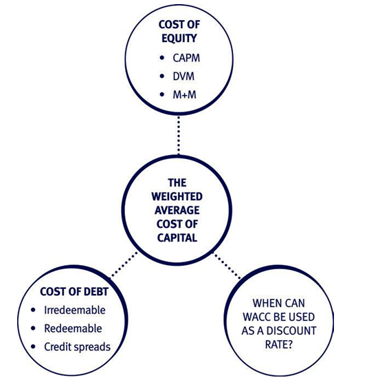
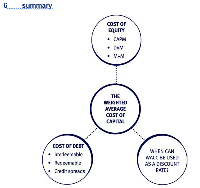
Overview of the WACC
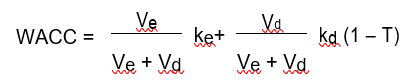
A key consideration in financial management is the firm’s WACC. The WACC is derived by finding a firm’s cost of equity and cost of debt and averaging them according to the market value of each source of finance. The formula for calculating WACC is given on the exam formula sheet as:
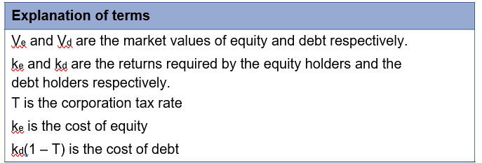
Explanation of terms
This reviews the basic techniques for deriving cost of equity and cost of debt from the Financial Management (FM) syllabus, and adds some more advanced techniques too.
This reviews the basic techniques for deriving cost of equity and cost of debt from the Financial Management (FM) syllabus, and adds some more advanced techniques too.
204
6
2 The cost of equity
Methods of calculating the cost of equity (ke)
The three main methods of calculating ke are:
- the Capital Asset Pricing Model (CAPM)
- the Dividend Valuation Model (DVM)
- Modigliani and Miller’s Proposition 2 formula.
The formulae for these methods are all given on the exam formula sheet.
The Capital Asset Pricing Model (CAPM)
The CAPM derives a required return for an investor by relating return to the level of systematic risk faced by an investor – note that the CAPM is based on the assumption that all investors are well-diversified, so only systematic risk is relevant.
The CAPM formula is:
Required return (ke) = Rf + ßi (E(Rm) – Rf)
where:
Rf = risk free rate
E(Rm) = expected return on the market
N.B. (E(Rm) – Rf) is called the equity risk premium
ßi = beta factor = systematic risk of the firm or project compared to market.
The portfolio effect
The CAPM model is based upon the assumption that investors are well diversified, so will have eliminated all the unsystematic (specific) risk from their portfolios. The beta factor is a measure of the level of systematic risk (general, market risk) faced by a well-diversified investor – see more details on beta factors below.
The risk reduction through diversifying is known as the portfolio effect.
If an investor is not well diversified, the level of risk affecting the investor can be calculated using the 2 asset portfolio formula:
Overall risk (standard deviation) = (w2a s2a + w2b s2b + 2wa wb rab sa sb)½
where
wa and wb are the proportions invested in two investments a and b
sa and sb are the risks associated with investments a and b (standard deviations)
rab is the correlation coefficient of the investments a and b
This formula is provided for information only. It is no longer examinable in AFM.
The beta factor
The beta factor indicates the level of systematic risk faced by an investor.
A beta > 1 indicates above average risk, while beta < 1 means relatively low risk.
Beta factors are derived by statistically analysing returns from a particular share over a period compared to the overall market returns. If the returns on the individual share are more volatile than the overall market, the firm’s beta will be greater than 1.
Illustration of the use of the CAPM formula
Gillespie Co has a beta factor of 1.73. The current return on a risk free asset is 3% per annum and the equity risk premium is 12%.
Hence, using CAPM, Gillespie Co’s cost of equity (return required by the shareholders) is 3% + (1.73 × 12%) = 23.76%.
Which beta factor to use?
To calculate the current cost of equity of a firm, the current beta factor can be used.
However, if the firm’s current beta factor cannot be derived easily, a proxy beta may be used.
A proxy beta is usually found by identifying a quoted company with a similar business risk profile and using its beta. However, when selecting an appropriate beta from a similar company, account has to be taken of the gearing ratios involved.
The beta values for companies reflect both:
- business risk (resulting from operations)
- finance risk (resulting from their level of gearing).
There are therefore two types of beta:
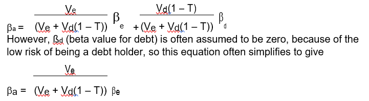
- ‘Asset’ or ‘ungeared’ beta, ßa, which reflects purely the systematic risk of the business area.
- ‘Equity’ or ‘geared’ beta, ße, which reflects the systematic risk of the business area and the company specific gearing ratio.
In the exam, you will often have to degear the proxy equity beta (using the gearing of the quoted company) and then regear to reflect the gearing position of the company in question.
The formula to regear and degear betas is:
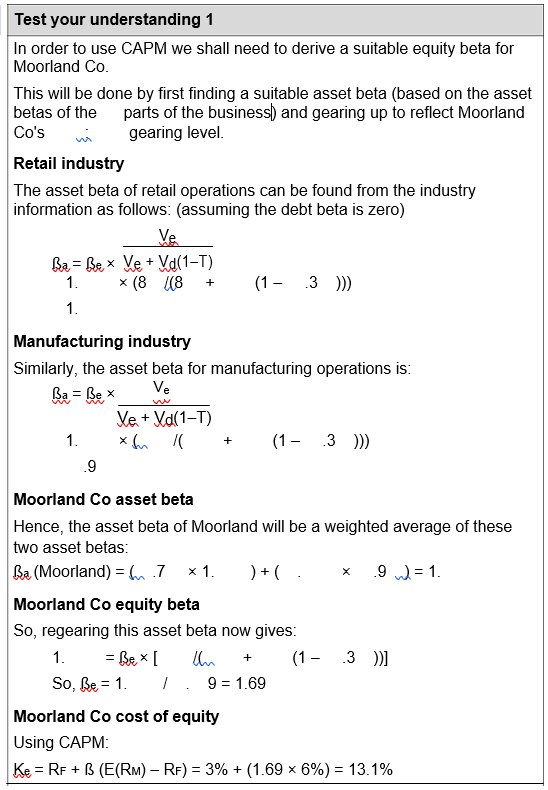
Test your understanding 1
The directors of Moorland Co, a company which has 7 % of its operations in the retail sector and % in manufacturing, are trying to derive the firm’s cost of equity. However, since the company is not listed, it has been difficult to determine an appropriate beta factor. Instead, the following information has been researched:
Retail industry – quoted retailers have an average equity beta of 1. , and an average gearing ratio of :8 (debt:equity).
Manufacturing industry – quoted manufacturers have an average equity beta of 1. and an average gearing ratio of : (debt:equity).
The risk free rate is 3% and the equity risk premium is 6%. Tax on corporate profits is 3 %. Moorland Co has gearing of % debt and % equity by market values. Assume that the risk on corporate debt is negligible.
Required:
Calculate the cost of equity of Moorland Co using the CAPM model.
Arbitrage pricing theory
Arbitrage pricing theory (APT) is an alternative pricing model to CAPM, developed by Stephen Ross in 1976. It attempts to explain the risk -return relationship using several independent factors rather than a single index.
CAPM is a single index model in that the expected return from a security is a function of only one factor, its beta value:
Expected return = Rf + ß (E(Rm) – Rf)
However APT is a multi-index model in that the expected return from a security is a linear function of several independent factors:
Expected return = a + ß1 f1 + ß f + …
where a, ß1, ß , … are constants
f1, f , … are the various factors that influence security returns
For example, f 1 could be the return on the market (as in CAPM), f could be an industry index specific to the sector in which the company operates, f3 could be an interest rate index, etc.
Ross showed that, if shares are assumed to form an efficient market, an equilibrium is reached when:
Expected return = Rf + ß1 (R1 – Rf) + ß (R – Rf) + …
where Rf = the risk free rate
ßi = constants expressing the security’s sensitivity to each factor
Ri = the expected return on a portfolio with unit sensitivity to factor i and zero sensitivity to any other factor.
Research undertaken to date suggests that there are a small number of factors, or economic forces, that systematically affect the returns on assets. These are:
- inflation or deflation
- long run growth in profitability in the economy
- industrial production
- term structure of interest rates
- default premium on bonds
- price of oil.
Each factor must be independent of the other factors. APT assumes that the process of arbitrage would ensure that two assets offering identical returns and risks will sell for the same price. Intuitively, APT appears to improve on CAPM, as return is determined by a number of independent factors. The main practical difficulties are in determining what those factors are, as the model does not specify them, and forecasting their value. There have been few tests of APT, probably because of the difficulties in determining which variables to include in the model and how to weigh them.
APT has gained in popularity as empirical tests of CAPM in practice have raised significant doubts as to CAPM’s validity. However it is fair to say that empirical testing of APT has to date been only limited, so its effectiveness remains to be proved. CAPM is certainly simpler than APT, being a single index rather than a multi-index model, so CAPM will remain popular for some time.
The dividend valuation model (DVM)
Theory: The value of the company/share is the present value of the expected future dividends discounted at the shareholders’ required rate of return.
Assuming a constant growth rate in dividends, g:
P = D (1 + g)/(ke – g)
(this formula is given on the formula sheet)
Explanation of terms
D = current level of dividend
P = current share price
g = estimated growth rate
If we need to derive ke the formula can be rearranged to:
ke = [D (1 + g)/P ] + g
Illustration of the DVM formula
Cocker Co has just paid a dividend of 1 cents per share. In recent years, annual dividend growth has been 3% per annum, and the current share price is $1. 8.
Using the DVM formula, the cost of equity is [ .1 × 1. 3/1. 8] + . 3 = 1 .7%.
Deriving g in the DVM formula
There are two ways of estimating the likely growth rate of dividends:
- Extrapolating based on past dividend patterns.
- Assuming growth is dependent on the level of earnings retained in the business.
Estimating dividend growth from past dividend patterns
This method assumes that the past pattern of dividends is a fair indicator of the future.
The formula for extrapolating growth can therefore be written as:
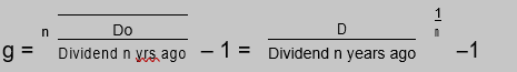
where:
n = number of years of dividend growth
This method can only be used if:
- recent dividend pattern is considered typical
- historical pattern is expected to continue.
As a result, this method will usually only be appropriate to predict growth rates over the short term.
Illustration of the calculation
A company currently pays a dividend of 3 ¢; five years ago the dividend was ¢.
Estimate the annual growth rate in dividends.
Solution
Since growth is assumed to be constant, the growth rate, g, can be assumed to have been the same in each of the years, i.e. the ¢ will have become 3 ¢ after years of constant growth.
¢ × (1 + g) = 3 ¢
or (1 + g) = 3 / = 1.6
1 + g = 1.61/ ≈ 1.1, so g = .1 or 1 %.
Estimating growth using the earnings retention model (Gordon’s growth model)
This model is based on the assumption that:
- growth is primarily due to the reinvestment of retained earnings The formula is therefore:
g = r × b where:
b = earnings retention rate r = rate of return to equity
What is r?
At FM level, r was considered to be the Accounting Rate of Return on equity calculated as:
r = PAT/opening shareholders’ funds
However, at AFM level we need to re-examine this assumption. The weakness of the ARR as a measure of return is that:
- it ignores the level of investment in intangible assets
- in the long run, the return on new investment tends to the cost of equity.
Hence, if a short term growth rate is required, the ARR provides a fair approximation for use in the growth model. However, if a long term growth rate is needed, ke should be used as the percentage return. To avoid a recursion problem, this should be derived using CAPM.
Modigliani and Miller’s Proposition formula
Modigliani and Miller’s gearing theory was covered in the earlier on the financing decision.
As part of their theory, they derived a formula which can be used to derive a firm’s cost of equity:
ke = kei + (1 – T)(kei – kd )(Vd / Ve)
(this formula is given on the formula sheet)
Explanation of terms
Ve and Vd are the market values of equity and debt respectively.
kd is the (pre-tax) return required by the debt holders.
T is the corporation tax rate.
kei is the cost of equity in an equivalent ungeared firm.
ke is the cost of equity in the geared firm.
Test your understanding
Moondog Co is a company with a :8 debt:equity ratio. Using CAPM, its cost of equity has been calculated as 1 %.
It is considering raising some debt finance to change its gearing ratio to :7 debt to equity. The expected return to debt holders is % per annum, and the rate of corporate tax is 3 %.
Required:
Calculate the theoretical cost of equity in Moondog Co after the refinancing.
3 The cost of debt
Methods of calculating cost of debt
The company’s cost of debt is found by taking the return required by debt holders/lenders (kd) and adjusting it for the tax relief received by the firm as it pays debt interest.
Note on exam terminology
In exam questions you may be given the cost of debt or you may have to calculate it – see below for calculations.
If you are given the ‘cost of debt’, be aware that the cost of debt is normally quoted pre-tax because this is the rate at which the companies will pay interest on their borrowings (even though the ‘true’ cost to them will be net of tax because interest is payable before tax and therefore companies benefit from the ‘tax shield’).
It can be assumed, therefore, that cost of debt will mean pre-tax cost of debt (kd) unless it is clearly stated otherwise.
Using the DVM to estimate cost of debt
In Financial Management (FM), the cost of debt was generally estimated using the principles of the dividend valuation model. As seen above, the basic theory of the DVM is:
The value of a share = the present value of the future dividends discounted at the shareholders’ required rate of return.
Using the same logic
The value of a bond = the present value of the future receipts (interest and redemption amount) discounted at the lenders’ required rate of return.
This theory gives rise to two alternative calculations of kd (1–T), for irredeemable debt and redeemable debt.
Irredeemable debt
kd (1–T) = I (1–T)/MV
where
I = the annual interest paid
T = corporation tax rate
MV = the current bond price
Test your understanding 3
Mackay Co has some irredeemable, % coupon bonds in issue, which are trading at $9 . per $1 nominal. The tax rate is 3 %.
Required:
Calculate Mackay Co’s post-tax cost of debt.
Redeemable debt
kd (1–T) = the Internal Rate of Return (IRR) of:
- the bond price
- the interest (net of tax)
- the redemption payment.
Test your understanding
Dodgy Co’s 6% coupon bonds are currently priced at $89%. The bonds are redeemable at par in years. Corporation tax is 3 %.
Required:
Calculate the post-tax cost of debt.
Pre-tax cost of debt (or ‘yield’ to the debt holder)
In both the previous examples, the focus was on finding the post-tax cost of debt, which is a key component in the company’s WACC calculation.
In order to compute the pre-tax cost of debt (sometimes called the yield to the investor, yield to maturity, or gross redemption yield) the method is very similar.
For irredeemable debt, the pre-tax cost of debt is simply I/MV.
For redeemable debt, the pre-tax cost of debt is the IRR of the bond price, the GROSS interest (i.e. pre-tax) and the redemption payment.
In both cases, the only difference from the above calculations is that interest is now taken pre-tax in the formulae.
Student Accountant article
The examiner’s article ‘Bond valuation and bond yields’ in the Technical Articles section of the ACCA website covers the calculation of bond yields in more detail.
Credit spread
An alternative technique used in AFM for deriving cost of debt is based on an awareness of credit spread (sometimes referred to as the ‘default risk premium’), and the formula:
kd (1–T) = (Risk free rate + Credit spread) (1–T)
The credit spread is a measure of the credit risk associated with a company. Credit spreads are generally calculated by a credit rating agency and presented in a table like the one below.
Credit risk, rating agencies and spread
What is credit risk?
Credit or default risk is the uncertainty surrounding a firm’s ability to service its debts and obligations.
It can be defined as the risk borne by a lender that the borrower will default either on interest payments, the repayment of the borrowing at the due date or both.
The role of credit rating agencies
If a company wants to assess whether a firm that owes them money is likely to default on the debt, a key source of information is a credit rating agency.
They provide vital information on creditworthiness to:
- potential investors
- regulators of investing bodies
- the firm itself.
The assessment of creditworthiness
A large number of agencies can provide information on smaller firms, but for larger firms credit assessments are usually carried out by one of the international credit rating agencies. The three largest international agencies are Standard and Poor’s, Moody’s and Fitch.
Certain factors have been shown to have a particular correlation with the likelihood that a company will default on its obligations:
- The magnitude and strength of the company’s cash flows.
- The size of the debt relative to the asset value of the firm.
- The volatility of the firm’s asset value.
- The length of time the debt has to run.
Using this and other data, firms are scored and rated on a scale, such as the one shown here:
| Fitch/S&P | Grade | Risk of default |
| AAA | Investment | Highest quality – zero risk |
| AA | Investment | High quality – v little risk |
| A | Investment | Strong – minimal risk |
| BBB | Investment | Medium grade – low but clear risk |
| BB | Junk | Speculative – marginal |
| B | Junk | Significant risk exposure |
| CCC | Junk | Considerable risk exposure |
| CC | Junk | Highly speculative – v high risk |
| C | Junk | In default – v high likelihood of failure |
Calculating credit scores
The credit rating agencies use a variety of models to assess the creditworthiness of companies.
In the popular Kaplan Urwitz model, measures such as firm size, profitability, type of debt, gearing ratios, interest cover and levels of risk are fed into formulae to generate a credit score.
These scores are then used to create the rankings shown above. For example a score of above 6.76 suggests an AAA rating.
Credit spread
There is no way to tell in advance which firms will default on their obligations and which won’t. As a result, to compensate lenders for this uncertainty, firms generally pay a spread or premium over the risk free rate of interest, which is proportional to their default probability.
The yield on a corporate bond is therefore given by:
Yield on corporate bond = Yield on equivalent treasury bond
+ credit spread
Table of credit spreads for industrial company bonds:
| Rating | 1 yr | yr | 3 yr | yr | 7 yr | 1 yr | 3 yr |
| AAA | 1 | 1 | 7 | 3 | |||
| AA | 1 | 3 | 37 | 6 | |||
| A | 7 | 6 | 71 | 7 | 9 | ||
| BBB | 6 | 8 | 88 | 9 | 1 6 | 1 9 | 17 |
| BB | 1 | 3 | 6 | 7 | 9 | ||
| B+ | 37 | 1 |
Examples of calculations of yield
Simple illustration
The current return on -year treasury bonds is 3.6%. C plc has equivalent bonds in issue but has an A rating. What is the expected yield on C’s bonds?
Solution
From the table the credit spread for an A rated, -year bond is 6 .
This means that .6 % must be added to the yield on equivalent treasury bonds.
So yield on C’s bonds = 3.6% + .6 % = . %.
More advanced illustration
The current return on 8-year treasury bonds is . %. X plc has equivalent bonds in issue but has a BBB rating. What is the expected yield on X’s bonds?
Solution
From the table the credit spread for a BBB rated, 7-year bond is 1 6. The spread for a 1 -year bond is 1 9.
This would suggest an adjustment of
| 1 6 + | (1 9 – 1 6) | |
| 3 | ||
= 1 6 + 7.67 = 133.67
So 1.3 % must be added to the yield on equivalent treasury bonds.
So yield on X’s bonds = . % + 1.3 % = . %.
Test your understanding
The current -year risk free return is .6%. F plc has -year bonds in issue but has a AA rating.
Required:
- calculate the expected yield on F’s bonds
- find F’s post-tax cost of debt associated with these bonds if the rate of corporation tax is 3 %.
(Use the information in the table of credit spreads above).
Test your understanding 6
Landline Co has an A credit rating.
It has $3 m of year bonds in issue, which are trading at $9 %, and $ m of 1 year bonds which are trading at $1 8%.
The risk free rate is . % and the corporation tax rate is 3 %.
Required:
Calculate the company’s post-tax cost of debt capital.
(Use the information in the table of credit spreads above).
More details on the ‘risk free rate’ – The spot yield curve
In all the previous examples, the risk free rate has been given as a single figure, based on the return required on government bonds.
However, in reality the return required will usually be higher for longer dated government bonds, to compensate investors for the additional uncertainty created by the longer time period.
Therefore, you might be given a ‘spot yield curve’ for government bonds, instead of a single ‘risk free rate’. Then to calculate the yield curve for an individual company’s bonds, add the given credit spread to the relevant government bond yield.
Test your understanding 7
The spot yield curve for government bonds is:
Year %
1 3.
3.6
3 3.8
The following table of credit spreads (in basis points) is presented by
Standard and Poor’s:
| Rating | 1 year | year | 3 year |
| AAA | 1 | 38 | |
| AA | 9 | 1 | |
| A | 6 | 6 | 76 |
Required:
Estimate the individual yield curve for Stone Co, an A rated company.
Estimating the spot yield curve
There are several different methods used to estimate a spot yield curve, and the iterative process based on bootstrapping coupon paying bonds is perhaps the simplest to understand. Discussion of other methods of estimating the spot yield curve, such as using multiple regression techniques and observation of spot rates of zero coupon bonds, is beyond the scope of the AFM syllabus.
The following example demonstrates how the iterative process works:
Illustration of how to calculate the spot yield curve for government bonds
A government has three bonds in issue that all have a par value of $1 and are redeemable in one year, two years and three years respectively. Since the bonds are all government bonds, let’s assume that they are of the same risk class. Let’s also assume that coupons are payable on an annual basis.
Bond A, which is redeemable in a year’s time, has a coupon rate of 7% and is trading at $1 3.
Bond B, which is redeemable in two years, has a coupon rate of 6% and is trading at $1 .
Bond C, which is redeemable in three years, has a coupon rate of % and is trading at $98.
To determine the spot yield curve, each bond’s cash flows are discounted in turn to determine the annual spot rates for the three years, as follows:
Bond A: $1 3 = $1 7/(1 + r1)
so r1 = 1 7/1 3 – 1 = . 388 or 3.88%
Bond B: $1 = ($6/1. 388) + [1 6/(1 + r ) ]
so r = [1 6/(1 – .78)]1/ – 1= . 96 or .96%
Bond C: $98 = ($ /1. 388) + ($ /1. 96 ) + [1 /(1 + r3)3]
so r3 = [1 /(98 – .81 – . )]1/3 – 1 = . 8 or .8 % The annual spot yield curve is therefore
Year %
1 3.88
.96
3 .8
Student Accountant article
The examiner’s article ‘Bond valuation and bond yields’ in the Technical Articles section of the ACCA website covers the calculation of bond yield curves in more detail.
Using the CAPM to calculate cost of debt
The CAPM can be used to derive a required return as long as the systematic risk of an investment is known. Earlier in the we saw how to use an equity beta to derive a required return on equity. We also said that the risk on debt is usually relatively low, so the debt beta is often zero. However, if the debt beta is not zero (for example if the company’s credit rating shows that it has a credit spread greater than zero) the CAPM can also be used to derive kd as follows:
kd = Rf + ßdebt (E(Rm) – Rf)
Then, the post-tax cost of debt is kd (1–T) as usual.
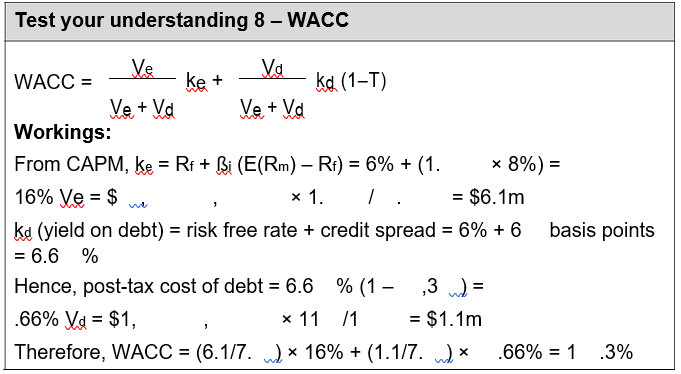
Test your understanding 8 – WACC
An entity has the following information in its balance sheet (statement of financial position):
| $ | |
| Ordinary shares ( c nominal) | , |
| Debt (8%, redeemable in years) | 1, |
The entity’s equity beta is 1. and its credit rating according to Standard and Poor’s is A. The share price is $1. and the debenture price is $11 per $1 nominal.
Extract from Standard and Poor’s credit spread tables:
| Rating | 1 yr | yr | 3 yr | yr | 7 yr | 1 yr | 3 yr |
| AAA | 1 | 1 | 7 | 3 | |||
| AA | 1 | 3 | 37 | 6 | |||
| A | 7 | 6 | 71 | 7 | 9 |
The risk free rate of interest is 6% and the equity risk premium is 8%. Tax is payable at 3 %.
Required:
Calculate the entity’s WACC.
Application of duration to debt
In , we saw how to calculate the Macaulay Duration and the Modified Duration of an investment project. The methods can also be used to measure the sensitivity of a bond’s price to a change in interest rates.
The bigger the duration, the greater the risk associated with the bond.
Illustration of duration calculation for a bond
Tyminski Co has some 1 % coupon bonds in issue. They are redeemable at par in years, and are trading at $97. %. The yield (pre-tax cost of debt) is 1 .7 3%.
The Macaulay Duration is calculated first, as follows:
Step 1: Calculate the present value of each future receipt from the bond, using the pre-tax cost of debt as the discount rate.
| ($) | t1 | t | t3 | t | t |
| Receipt | 1 | 1 | 1 | 1 | 11 |
| PV @ 1 .7 3% | 9. 3 | 8.1 | 7.36 | 6.66 | 66. |
Step : Calculate the sum of (time to maturity × PV of receipt)
(1 × 9. 3) + ( × 8.1 ) + (3 × 7.36) + ( × 6.66) + ( × 66. ) = .3
Step 3: Divide this by the total PV of receipts (i.e. the bond price) to give the Macaulay Duration.
Macaulay Duration = .3 /97. = .1 7 years
The longer the Macaulay Duration, the more volatile the bond.
Modified Duration
Note that the Modified Duration can then be simply calculated as:
Macaulay Duration/(1 + discount rate)
- .1 7/1.1 7 3
The size of the Modified Duration identifies how much the value of the bond will change if there is a change in interest rates. A higher modified duration means that the fluctuations in the value of the bond will be greater, hence the value of 3.7 means that the value of the bond will change by 3.7 times the change in interest rates multiplied by the original value of the bond.
The relationship is only an approximation because duration assumes that the relationship between the change in interest rates and the corresponding change in the value of the bond or loan is linear. In fact, the relationship between interest rates and bond price is in the form of a curve which is convex to the origin (i.e. non-linear). Therefore duration can only provide a reasonable estimation of the change in the value of a bond or loan due to changes in interest rates, when those interest rate changes are small.
Benefits and limitations of duration
Benefits
- Duration allows bonds of different maturities and coupon rates to be compared. This makes decision making regarding bond finance easier and more effective.
- If a portfolio of bonds is constructed based on weighted average duration, it is possible to identify the change in value of the portfolio as interest rates change.
- Managers may be able to reduce interest rate risk by changing the overall duration of the bond portfolio (e.g. by adding shorter maturity bonds to reduce duration).
Limitations
The main limitation of duration is that it assumes a linear relationship between interest rates and bond price. In reality, the relationship is likely to be curvilinear. The extent of the deviation from a linear relationship is known as convexity. The more convex the relationship between interest rates and bond price, the more inaccurate duration is for measuring interest rate sensitivity.
Further information on convexity
The sensitivity of bond prices to changes in interest rates is dependent on their redemption dates. Bonds which are due to be redeemed at a later date are more price-sensitive to interest rate changes, and therefore are riskier.
Duration measures the average time it takes for a bond to pay its coupons and principal and therefore measures the redemption period of a bond. It recognises that bonds which pay higher coupons effectively mature ‘sooner’ compared to bonds which pay lower coupons, even if the redemption dates of the bonds are the same.
This is because a higher proportion of the higher coupon bonds’ income is received sooner. Therefore these bonds are less sensitive to interest rate changes and will have a lower duration.
Duration can be used to assess the change in the value of a bond when interest rates change using the following formula:
∆P = [–D × ∆i × P]/[1 + i],
where P is the price of the bond, D is the duration and i is the redemption yield.
However, duration is only useful in assessing small changes in interest rates because of convexity. As interest rates increase, the price of a bond decreases and vice versa, but this decrease is not proportional for coupon paying bonds, the relationship is non-linear. In fact, the relationship between the changes in bond value to changes in interest rates is in the shape of a convex curve to origin, see below.
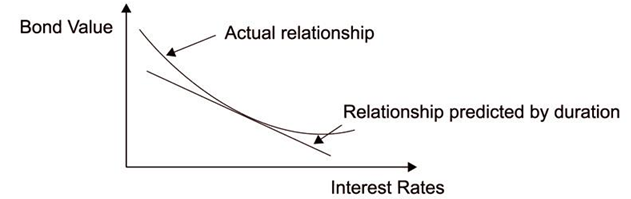
Duration, on the other hand, assumes that the relationship between changes in interest rates and the resultant bond is linear.
Therefore duration will predict a lower price than the actual price and for large changes in interest rates this difference can be significant. Duration can only be applied to measure the approximate change in a bond price due to interest changes, only if changes in interest rates do not lead to a change in the shape of the yield curve. This is because it is an average measure based on the gross redemption yield (yield to maturity). However, if the shape of the yield curve changes, duration can no longer be used to assess the change in bond value due to interest rate changes.
How do lenders set their interest rates?
Link to credit spreads
The table of credit spreads shown above showed the premium over risk free rate which a company would have to pay in order to satisfy its lenders. Another way of looking at the issue of yield on a bond is to look at it from the perspective of the lender.
Overview of the method
Lenders set their interest rates after assessing the likelihood that the borrower will default. The basic idea is that the lender will assess the likelihood (using normal distribution theory) of the firm’s cash flows falling to a level which is lower than the required interest payment in the coming year. If it looks likely that the firm will have to default, the interest rate will be set at a high level to compensate the lender for this risk.
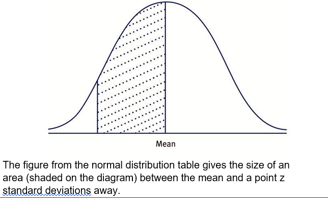
Introduction to normal distribution theory
The exam formula sheet contains a normal distribution table. Normal distributions have several applications in the AFM syllabus.
A normal distribution is often drawn as a ‘bell shaped’ curve, with its peak at the mean in the centre, as shown:
Example of a simple normal distribution
The height of adult males is normally distributed with a mean of 17 cm and a standard deviation of cm.
What is the probability of a man being shorter than 168cm?
Solution
168cm is 7cm away from the mean.
This represents 7/ = 1. standard deviations.
From tables, . 19 of the normal curve lies between the mean and 1. standard deviations.
Hence, the probability of a man being shorter than 168cm is . – . 19 = . 8 8 (approximately 8%).
Illustration of how lenders set their interest rates
Villa Co has $ m of debt, on which it pays annual interest of 6%.
The company’s operating cash flow in the coming year is forecast to be $1 , , and currently the company has $1 , cash on deposit.
Required:
Given that the annual volatility (standard deviation) of the company’s cash flows (measured over the last years) has been %, calculate the probability that Villa Co will default on its interest payment within the next year (assuming that the company has no other lines of credit available).
Solution
The key here is that Villa Co will have expected cash of $1 , + $1 , = $1 , , and its interest commitment will be 6% on $ m, i.e. $1 , .
We need to calculate the probability that the cash available will fall by $1 , – $1 , = $3 , over the next year.
Assuming that the annual cash flow is normally distributed, a volatility (standard deviation) of % on a cash flow of $1 , represents a standard deviation of . × $1 , = $3 , .
Thus, our fall of $3 , represents 3 , /3 , = .91 standard deviations.
From the normal distribution tables, the area between the mean and .91 standard deviations = .3186.
Hence, there must be a . – .3186 = .181 chance of the cash flow being insufficient to meet the interest payment.
i.e. the probability of default is approximately 18%.
The use of WACC as a discount rate in project appraisal
Link to project appraisal
When evaluating a project, it is important to use a cost of capital which is appropriate to the risk of the new project. The existing WACC will therefore be appropriate as a discount rate if both:
- the new project has the same level of business risk as the existing operations. If business risk changes, required returns of shareholders will change (to compensate them for the new level of risk), and hence WACC will change.
- undertaking the new project will not alter the firm’s gearing (financial risk). The values of equity and debt are key components in the calculation of WACC, so if the values change, clearly the existing WACC will no longer be applicable.
If one or both of these factors do not apply when undertaking a new project, the existing WACC cannot be used as a discount rate. The next explores the alternative methods available in these situations.
Test your understanding
Using M+M’s Proposition equation, we can degear the existing ke and then regear it to the new gearing level:
Degearing:
ke = kei + (1 – T)(kei – kd)(Vd/Ve)
1 % = kei + (1 – .3 )(kei – % )( /8 )
Now we need to rearrange this formula:
.1 = kei + (1- .3 )( kei – . )( /8 )
.1 = kei + ( .7)( kei – . )( . )
.1 = kei + ( .17 )( kei – . )
.1 = kei + .17 kei – . 7
.1 = 1.17 kei – . 7
.1 7 = 1.17 kei
( .1 7/1.17 ) = kei
So rearranging carefully gives kei = .1 8 (1 .8%)
Now regearing:
ke = 1 .8% + (1 – .3 )(1 .8% – %)( /7 )
ke = 1 . %
Test your understanding 3
Mackay Co’s post-tax cost of debt is (1 – .3 )/9 . = 3.7%
Test your understanding
To calculate IRR, we discount at rates ( % and 1 % here) and then interpolate:
PV at % = 89 – (6(1 – .3 ) × yr % annuity factor) – (1 × yr % discount factor) = –7. 8
PV at 1 % = 89 – (6(1 – .3 ) × yr 1 % annuity factor) – (1 × yr 1 % discount factor) = 1 .98
Hence IRR (post-tax cost of debt) is approximately
- % + (–7. 8/(–7. 8 – 1 .98) × (1 % – %))
- %
Test your understanding
From the table the credit spread for an AA rated, 3-year bond is 3 . The spread for a -year bond is 37.
This would suggest an adjustment of:
3 + (37 – 3 )/ = 33. basis points
The yield is therefore found by adding .33 % to the risk free rate.
So yield on F’s bonds =
.6% + .33 % = .93 %
The cost of debt = .93 × (1 – .3) = . %.
Test your understanding 6
The overall cost of debt will be the weighted average of the costs of the two types of debt (weighted according to market values).
year bonds
Market value = $3 m × .9 = $ 7m
kd = . % + credit spread (from table) = 3. %
1 year bonds
Market value = $ m × 1. 8 = $ m
kd = . % + 7 credit spread (from table) = 3. %
Overall cost of debt
Therefore the weighted average cost of debt (given that the ratio of market values is 1: ) is
[((1/3) × 3. %) + (( /3) × 3. %)] × (1 – .3 ) = . %
Test your understanding 7
The individual yield curve for Stone Co is found by adding the government spot yield curve figures to the credit spreads for an A rated company:
| Year | Spot yield (%) | Credit spread | Individual yield |
| (%) | curve (%) | ||
| 1 | 3. | . 6 | 3.96 |
| 3.6 | .6 | . | |
| 3 | 3.8 | .76 | . 6 |
This shows that (for example) the yield on a year Stone Co bond will be . %.