
THE NATURE OF PROFIT
The simplest definition of profit is that it is the excess of revenue over cost. This is a little deceptive because it is not always easy, in practice, to decide what is revenue and what is cost, and there are also problems arising from changes in the value of property. For example, the value of a building may rise or fall for reasons that have nothing to do with the trade carried on in that building. At this stage, however, it is convenient to overlook problems of this kind and keep simply to the idea of profit as the excess of the revenue gained by selling products over the cost of producing those products.
Nevertheless the above definition does not satisfy the economist’s desire to explain why profit exists and what its economic function really is; and here we come up against two rather conflicting ideas. On the one hand there is what might be called the traditional view of profit as a payment to a factor of production, just as wage is the payment to labour or rent the payment to capital; while on the other there is the view that profit is surplus which remains when the payments to production factors have all been made. Both views present difficulties as we shall now see.
Profit as a Factor Payment
Although considered by many as being rather old-fashioned and difficult to reconcile with modern realities, this is the view which still dominates most of the basic economics text books and, as far as it is possible to tell, the thinking of most of today’s examiners of economics in the professional examinations. You must, therefore, take it into account. Attempts to reconcile the idea of profit as a factor payment with the reality that it is very uncertain and subject to all kinds of pressures, as well as being impossible to predict or guarantee, have resulted in the development of the concepts of “normal” and “abnormal” profit.
Normal and Abnormal Profit
Here profit is seen as a payment to a fourth factor of production, the factor “enterprise” provided by entrepreneurs, people who take economic risks by organising and combining the other factors to produce goods and services for sale in the markets. Normal profit is, thus, frequently described as the reward to the entrepreneur – an attractive idea, but one which raises many difficulties.
- How do we quantify “normal”? The usual answer to this question is to suggest that it is the minimum necessary to keep the entrepreneur in the market. However, this surely depends as much on conditions in other possible markets as on the amount of profit available in the one under scrutiny. Firms that have been operating in a particular market for a lengthy period, or which operate in that market only, face greater costs of transfer to another market than newcomers, especially those which already operate in many markets. Thus, the minimum required to keep firm A in the market is unlikely to be the same amount as that sought by firm B. As economics have become more and more precise, scientific and mathematical, fewer people have been prepared to accept a concept as vague and unquantifiable as “normal” profit, in this sense.
- Why is the entrepreneur entitled to “normal” profit? The early economists who developed the concept were accustomed to markets containing small, individually owned and controlled firms, so that the entrepreneur who was the driving force behind the firm was usually identifiable without much trouble.
Modern markets, on the other hand, are dominated by large, corporate organisations with clear, bureaucratic, managerial structures. The success of this type of enterprise may lie as much in the ability of managers to reduce risks as to take them and, while individual managers may be expected to show enterprise in their work, this is rarely rewarded directly with a proportionate share in profits – even if the profit attributable to the enterprise shown could be calculated. The statistical profit of the organisation belongs legally to the ordinary shareholders, who are specifically denied any right to share in management and who rarely have much detailed knowledge of the activities of the organisation. When we further recognise that the large public company, today, is likely to operate in many markets, in many countries, we have to agree that all this is impossible to reconcile with the definition of “normal profit”.
If, however, it is accepted that there is such a thing as normal profit then this implies that there can be “abnormal” profit. Some text books do, in fact, describe all profits above the normal as abnormal. Others, clearly unhappy at the emotive implications of this term, use the less derogatory “supernormal”. In either case, the impression is usually given that firms should not be permitted to earn profits above normal.
Instead of either abnormal or supernormal, some writers have referred to what they call “pure profit”, by which they appear to mean any surplus over and above all payments to factors including the “normal” profit due to the entrepreneur.
Profit as a Surplus
If we see profit not as a factor payment but as a surplus remaining after the production factors have been paid for, the question then arises as to who owns, or should own, this surplus.
To Marxist economists the answer is clear. Economic value is created by human labour, without which there can be no economic activity. The berries growing wild on the bush belong to the picker, whose labour of picking has turned them into food. Thus any surplus created by work belongs to those who carry out the work. Profit, therefore, to the Marxist who does not recognise a separate entrepreneur, belongs to the workers. However, the Marxist recognises that, in the modern capitalist society where production is organised by the owners of capital and, in the Marxist view, for the benefit of the owners of capital, profit is, in practice, allocated to the owners of capital.
If this view is accepted, profit, not interest, becomes the payment to the owners of capital. To the Marxist, the fact that it is paid to the owners of capital rather than to the rightful owners, the contributors of labour, is the result of the domination of capital over labour in the modern capitalist society.
In support of this view it is possible to point to company law, which provides that a company’s profit belongs to the company’s shareholders or, more precisely, to the contributors of the “risk capital” or “equity”, the ordinary shareholders – in American terminology, the common stock holders. There is no legal requirement that the company should share its profits with the suppliers of labour (employees) or with the suppliers of loan capital, who receive their agreed rate of interest.
Still largely accepting this concept of profit as a surplus other economists, some of whom belong to what has been called the “Austrian school”, take a very different view of its economic function. They see it as the driving force of the modern economy and the incentive which has been largely instrumental in bringing about the enormous improvement in general living standards in the market economies over the past two centuries. They see the striving for profit as the force that produces new products, new production technology, new forms of business organisation and new uses for basic resources. The profit that produces this economic energy and invites people of all kinds to take risks with their own resources of money, time and futures, is not “normal profit” but the largest possible profit that can be made in the circumstances within which business operates. There is no need to distinguish between normal and abnormal profit. All profit is necessary to stimulate future economic activity and to provide the investment finance necessary to make the activity possible and raise the level of technology.
Unlike Marxists, the economists who take this view do not see profit as being stolen from workers, nor do they see any need for labour to be given only the lowest possible wage. Indeed for business enterprise to succeed, goods and services have to be sold to workers whose incomes are well above subsistence levels, who have disposable incomes and the freedom to choose how to spend these incomes and who expect to have rising incomes. Workers therefore, benefit from profitable economic activity by earning rising wages.
Summary of Explanations of Profit
One economist who recognised the various ways in which profit has been explained was the great American writer and teacher, Professor Samuelson. He identified six distinct “views”, which can be summarised as follows:
- Profit is seen as a balancing item and a result of accounting conventions but should properly be seen as a return to one or more of the production factors. For example, most of what accountants show as the “profit” of the majority of small family firms would better be described as the proprietor’s wage for his physical and mental effort and interest on his personal savings invested in the business.
- The second view sees profit as a reward to “enterprise and innovation” and a return for the temporary monopoly achieved by being first in the field with a successful new commercial idea.
- The third sees profit as a reward for successful risk-taking and, although willingness to take risks does not always (or often) bring compensating profits, it is usually the hope of earning such profits that provides the spur to help business people overcome their natural inclination to avoid risk.
- The fourth view simply takes the third view further; profit is a positive incentive to “coax out the supply of risk-bearing capital”. It is the high return sought by providers of what is often known as “venture capital”.
- The fifth view regards profit as a return to monopoly, whether natural or achieved by artificial means. It is this association of “abnormal” profit with monopoly that has coloured so much teaching about business profits and objectives.
- The sixth view recognises the Marxist explanation of profit as surplus value which, for Marx, is properly the reward of the labour that created the value but which, in a capitalist economy, is appropriated by the owners of capital.
Clearly there is no simple or generally agreed explanation of the economic function of profit, though most would agree that both profit and a spirit of enterprise are extremely important elements in modern market economies.
MAXIMISATION OF PROFIT
Calculation
We can arrive at the amount of profit for any given level of output in at least two ways. We can calculate total revenue and total cost and find the difference, or we can calculate the average revenue and the average cost, find the difference and multiply this by the quantity sold.
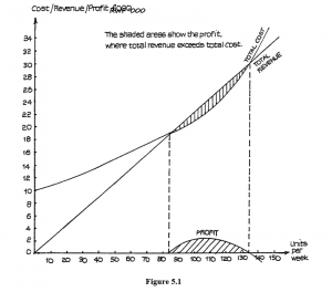
We shall first consider profit as the difference between total revenue and total cost. Suppose we return to the example of the last study unit and assume that all units of the product are sold at a given market price of RWF210 per unit. Costs remain as before. We can now show total revenue and cost columns for each range of output up to 150 units per week – as in Table 5.1.
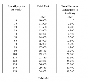
From this table we can see that revenue exceeds total cost at output levels 90 to 130 units per week. At all other output levels, total costs are greater than total revenue, so losses would be suffered.
The following table shows the profit at each output level.
Quantity Profit
RWF
90 750
100 1,500
110 1,950 120 1,950
130 1,300
The position is illustrated in Figure 5.1, where the shaded area represents the profit produced when total revenue is greater than total cost.
The same position is shown by the average cost and price/average revenue curves of Figure 5.2. In this case, however, the shaded area does not represent the total profit but the profit per unit of output. Total profit would be given by multiplying the profit per unit by the number of units produced.
In this example, the firm is selling all units at a given price, so that the total revenue curve continues to increase – though this does not, of course, mean that it is possible to make a profit at output levels above 130 or so units per week.
We saw in an earlier study unit that the revenue position could be rather different where the firm had to reduce price in order to increase output. Such a situation is illustrated in Figure 5.3. No figures are shown here – this is a general model – and it shows that the firm can make profits at all output levels between 0a and 0b.
These levels, where total revenue just equals total cost, are called the break-even output levels or sometimes “break-even points”.
It is often more convenient, however, to show the average cost and revenue curves (see Figure 5.4).
If we assume that the firm is selling all units at any given output level at the same price, i.e. is not discriminating between different customers over price, then the average revenue curve is also the price/output curve, i.e. the demand curve. In this model, we can also see that the firm makes profits between output levels 0a and 0b. This is the quantity range where average revenue is greater than average cost.
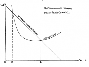
Figure 5.4
Profit Maximisation
So far, we have seen the output levels where profits are made, but we have not yet identified the output level where the largest possible (maximum) profit can be made. However, if we refer back to our profit table, we see that there are two points where points are at their largest – at output levels of 110 and 120 units per week. Here, total profit stays at RWF1,950. If the firm wants to make the largest possible profit, it can choose either of these two levels. It is not unusual for profit to have a rather “flat top” and stretch across two stages in this way. In other cases it can peak at a single stage.
Now look back at Table 4.1 in the last study unit, which showed marginal costs. Bearing in mind that we assumed the firm to be selling at a constant price of RWF210, look at the marginal cost column. We have explained that, when the firm can sell at a constant price at all levels of output, the price is also the average and the marginal revenue. Thus, in this case, the firm’s marginal revenue is RWF210. If you look down column 4, you will see that the marginal cost is RWF210 at the mid-point, representing the change from output level 110 to 120 units per week. This is precisely the output range where profits are at their highest level, i.e. RWF1,950.
This is no accident. It illustrates the general rule that profits are always maximised at the output levels where marginal cost is equal to marginal revenue.
The general position is illustrated in Figures 5.5 and 5.6. Figure 5.5 shows the case where average revenue = marginal revenue (constant price at all output levels) and Figure 5.6 shows the sloping average revenue curve with the marginal revenue curve in the correct position, as we explained before.
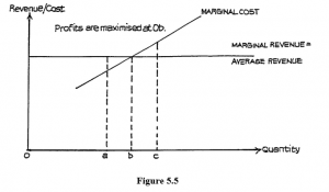
Figure 5.5
In both cases, the argument is the same. It does not matter whether the marginal revenue curve slopes or not. If the firm produces at output level 0a, i.e. below the level where marginal cost = marginal revenue, it would pay it to increase output because the revenue received for each additional unit is greater than the cost of producing that unit. If the firm is producing at output level 0c, above the level where marginal cost = marginal revenue, then it will pay it to reduce output because revenue lost for each unit of output sacrificed is less than the cost of its production. Only at output level 0b, where marginal cost = marginal revenue, will it pay the firm to stay at the same level. It cannot then increase profit by any change in quantity produced. This is the level where profits are maximised.
This is a most important rule which you should remember carefully, i.e. to maximise profits the firm produces at the output level where marginal cost is equal to marginal revenue.
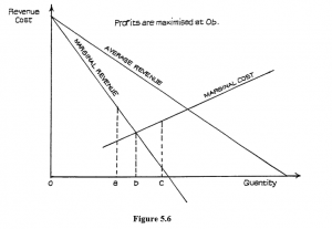
Figure 5.6
Do Firms Maximise Profits?
It is often argued that we should not automatically assume firms do seek to maximise profit. It is suggested that they may have other objectives, e.g. to maximise revenue, to increase output or to achieve a given share of the market, or simply to please and reconcile the conflicting objectives of shareholders, managers and employees.
All this may be true – many firms may not be seeking to maximise their profits. Many may not have sufficient information about market demand and their costs to profit-maximise even if they wished. On the other hand, this does not rule out our view that the profit-maximising output level and the rule for achieving this are matters of very great importance for an understanding of business decisions. The firm may decide to sacrifice some profit in order to pursue some other objective, but it should know how much profit is being sacrificed.
An assumption of profit-maximising behaviour is an essential starting point for the analysis of the business organisation. As long as we recognise that it is not necessarily the finishing point, then we can accept this assumption at this stage of our studies unless there is a very good reason to do otherwise.
INFLUENCES ON SUPPLY
Costs and Supply
If we accept that business firms exist to make profits, then we can recognise that there must be a close link between costs, profits and the willingness of firms to produce the goods and services that consumers wish to buy. After all, profit is the difference between revenue and costs, so that at any given price the amount of profit will depend on production costs. If price remains constant and costs rise, then profit falls and we can expect firms to be less willing to supply goods and services. Similarly, if costs remain unchanged and price rises, then profits will rise and firms will wish to supply more in order to secure the increased profit.
We thus have no difficulty in accepting the link between costs and the amount that firms are prepared to supply at a given price or range of prices. If we accept the aim of profit maximisation, then we can be a little more precise than this.
Suppose a firm is seeking to maximise profits and can sell all it can produce at the ruling market price. Suppose, too, that this market price can change. What, then, will be the firm’s response? Look at Figure 5.7. The profit-maximising firm will seek to produce at that output level where marginal cost is equal to price, i.e. at quantity 0q at price 0p, at 0q1 at price 0p1, and 0q2 at price 0p2.
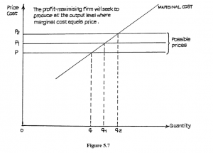
Figure 5.7
Thus, we can see that the firm will increase the quantity it is willing to supply as price increases – and, conversely, reduce quantity as price falls – and that the actual change in quantity will be governed by the marginal cost curve.
Under conditions of perfect competition, therefore, the individual firm’s supply curve is its marginal cost curve and, consequently, the market supply curve is derived from the sum of the marginal cost curves of all the firms operating within the market.
This argument continues to hold good when we abandon the assumption of the firm accepting the market price. If the firm faces a downward-sloping demand curve for its product, and hence a downward-sloping marginal revenue curve, we still get the same increase in quantity following the marginal cost curve if we again move the marginal revenue curve outwards, further from the point of origin. This is shown in Figure 5.8.
Notice, however, that Figure 5.8 is drawn on the assumption that the average revenue curve is moving outwards evenly and with its slope unchanged. There is no guarantee that this will ever happen in practice. If the slope of the average revenue curve changes, then so too will the slope of the marginal revenue curve, and there will no longer be the smooth increase in quantity suggested by Figure 5.8. For this reason, we cannot say that, in imperfect markets, the market supply curve will represent the sum of the marginal cost curves of the individual firms. Nevertheless, the general link between supply and marginal costs remains, although it is unlikely to be as direct as in perfect competition.
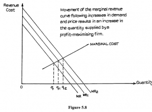
Figure 5.8
Here again, a movement of the marginal revenue curve produces a shift in quantity supplied, in accordance with the marginal cost curve.
You can, if you wish, add the average revenue curves to this graph, and thus show the prices corresponding to the three quantity levels 0q, 0q1 and 0q2. Remember the relationship between average and marginal revenue, and remember that price will be shown by the vertical line from any given quantity level to the average revenue curve.
Supply Curve
If we accept this view that firms will seek to increase the quantity supplied if price increases, and reduce it if price falls, then we can produce a supply curve showing the amounts involved. A supply curve can be for an individual firm – in which case, assuming profitmaximising objectives, it will be the marginal cost curve – or for all firms supplying a particular product, where it will be made up of the sum of the marginal cost curves of all the firms supplying the product.
However the supply curve is formed, we can accept that its general shape will be as in Figure 5.9. This shows the general assumption that more will be supplied as the price rises – all other influences remaining the same.
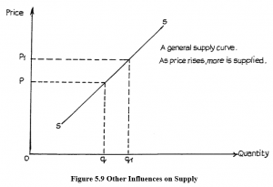
Figure 5.9 Other Influences on Supply
The concept of the supply curve reflects the view that price is one of the most important influences on the quantity supplied. There are other influences, however, and these are mostly concerned with the cost of production and with profits. Remember that, in a market economy, the great driving force for supply is profit, so anything that affects profit will affect supply. In very broad terms, since profit is the difference between revenue and costs, supply will be directly affected by anything affecting revenue, price and costs.
We can summarise some of the most important influences as follows:
Costs of Factors and Other Inputs
Any change in costs, with price staying constant, will change the profit expectations and will thus influence decisions regarding supply. For the profit-maximising firm, a change in variable costs will change the marginal cost curve, and so change the supply schedule. Examples of factor costs include wages, land and property rents, interest rates on capital, basic material prices and the prices of fuel and power. Any of these may also affect the prices of intermediate products and services required by the firm, and so further influence supply.
Changes in Taxes
If a tax, payable to the government, is charged at any stage of production or on the profits of the business, then any change in the tax rate will affect the profits anticipated from supply, and thus affect supply intentions. An increase in a production tax, such as value added tax, will have the same effect as an increase in factor costs; it will tend to reduce the quantity that firms are willing to supply at all prices in a given range.
Changes in Technology
By “technology” is meant the methods of combining factors and inputs in order to achieve production. An improvement in technology, which allows a given level of production to be achieved with fewer factor inputs or with a different combination of factors, so that the total cost is lower, will tend to increase the quantity likely to be supplied at all prices within the range. Some types of technology may be possible only if production is required on a large scale. This can have a marked effect on supply. Thus, small-scale supply may be possible only at much higher prices than large-scale supply, when the different technology becomes worthwhile. The result may be to shift the whole supply curve when production reaches the critical level required for the large-scale technology.
Efficiency of the Firm
Multinational production of similar products has shown that firms in country A can sometimes produce more from a given combination of labour and capital than similar firms in country B, even though production methods and levels of technology are all much the same. Differences in the productivity of labour and capital (the amount produced per unit of labour and capital) must, in these cases, be caused by differences in managerial efficiency or in the conditions under which people work. In some cases, the movement of managers from one country to the other makes little difference to the gap in factor productivity. The causes of these differing levels of efficiency are not fully understood, but they do help to explain why large multinational firms tend to prefer some countries to others. A change in the level of business efficiency will, of course, influence supply.
Changes in Relative Profitability of Products
If a firm can produce either product X or product Y from similar factors, machines and skills, and if it becomes more profitable to produce Y, then the firm is likely to switch its production activities from X to Y. This may happen if the firm normally makes X, but the price of Y rises while the price of X stays the same.
There can be other causes of production switches. If there are numbers of firms able to choose between producing X or Y, and the market for Y suddenly disappears, perhaps because of a political decision, then firms previously making Y will have to switch to X if they wish to remain in business. The result will be to increase the supply of X at all prices.
Effect of Other Influences on Supply Curve
All the above changes can be illustrated by a movement of the whole supply curve, indicating a change in supply intentions throughout the given price range. Such a shift in the supply curve is illustrated in the general graphical model of Figure 5.10.
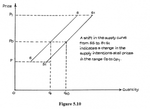
Figure 5.10
A shift of this type may follow a change in one or more of the influences as described above. Moreover, several influences may be operating, in different directions. For example, a tax increase may be depressing supply intentions while an improvement in technology is raising them. The final result depends on the relative strength of the influences. It is not easy to analyse these effects through simple graphical models. This is why more advanced studies make rather more use of algebraic models which can be easily handled by computers, and why you should begin to become familiar with functional expressions such as the following:
Qs = f(P, C, T, v, y, πo )
where Qs = quantity of a product supplied
P = product’s price
C = factory and input costs T = business taxes v = level of technology y = level of business efficiency
πo = relative profitability of products
This simply states that quantity supplied is a function of, or is dependent on, the various influences symbolised.
Relative Importance of Supply Influences
As with demand, different products will be affected to different degrees by the various influences on supply. In the case of supply, much will depend on the methods of production and the ease with which producers can respond to changes in factor costs and availability as well as in technology. Consequently, it is easier to assess the relative importance of the supply influences than those on demand. A careful study of production technology and relative factor costs will indicate which are likely to have the most impact on producer intentions. A production process heavily dependent on labour (labour-intensive) will be more responsive to changes in wage levels than one that is highly mechanised or automated and thus capital-intensive. On the other hand, production which is highly capital-intensive will be more vulnerable to changes in interest rates, since much capital is likely to be borrowed in one form or another. The potential costs of changing production levels tend to be greater with capital-intensive production methods.
PRICE ELASTICITY OF SUPPLY
Calculation of Elasticity
The concept of elasticity, which we applied to demand, can also be applied to supply. However, here it is usually only price elasticity with which we are concerned. The method of calculating supply elasticity is exactly the same as for price elasticity of demand, i.e.
Supply elasticity of a product (Es) = Proportional change in quantity supplied Proportional change in the product’s price
or Es= ∆Qs ÷∆P = P∆Qs
Qs P Qs∆P
Notice that the value of Es is always positive (+). This is because the change of quantity is in the same direction as the change in price.
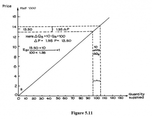
Figure 5.11 shows an example of a simple supply-elasticity calculation.
Notice here that figures for both P and Q are obtained from the mid-point of the change in price and quantity, so that the calculation is the same for both a rise and a fall in price. Notice also that the result of this particular calculation is that Es = unity (1).
If you calculate values for Es at any other price level on this curve, you should obtain the same results. The reason for this is explained in the next subsection.
Elastic and Inelastic Supply Curves
Price elasticity of demand was shown to change as price changed. A rather different position obtains in the case of supply elasticity. We said that the value of Es for the supply curve of Figure 5.11 would always be 1. This is because the curve starts at the point of origin.
A simple proof follows, relating to Figure 5.12, and assuming a knowledge of simple geometry.
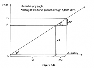
From the diagram:
θ=θ1and QP = tan θ
and ∆QP = tan θ1 ∆
so P = ∆P .
Q ∆Q
But Es = ∆QQ ÷∆PP = ∆QQ × ∆PP
- ∆Q
= ×
- ∆P
so QP ×∆∆QP = 1and Es = 1.
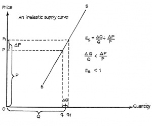
A supply curve which passes through the vertical (price) axis is elastic, and one which passes (or, if extended, would pass) through the horizontal (quantity) axis is inelastic. This holds regardless of the slope of the curve, and it applies to the whole curve when this is linear (forming a straight line).
These statements can be proved by the same method as in Figure 5.12. Don’t worry if you can’t prove them yourself – just remember the position. Examples are given in Figures 5.13
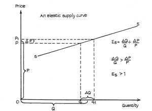
Figure 5.15
When the curve is non-linear, the important point is the direction of the tangent to the curve at the price level under consideration. This is shown in Figure 5.15.
Elasticity of Supply in the Long Run
The main influence on the elasticity of supply is the speed with which producers can respond to changes in cost, price and profitability. Few firms can alter their production plans immediately when basic materials, capital and labour have already been committed to them. As time goes on, however, plans can be changed, workers can be hired or fired, and new machines bought or old ones scrapped.
The speed and ease with which production plans can be changed depends on the nature of the production process. As a general rule processes, such as services, which are labour-intensive can be changed more quickly than those that are capital-intensive. Workers, especially if they are part-time can have their working hours increased or reduced and the number of workers employed can be changed, whereas capital-intensive processes, such as motor-vehicle assembly lines, still have to pay costs of capital even when equipment is no longer used. It may, therefore, be better to maintain production as long as variable costs are covered by sales revenue and there is some contribution to unavoidable fixed costs rather than suffer the heavy losses of a major production change. When, however, the decision has to be made to reduce production the consequences can be swift and far-reaching, with large numbers of workers suffering redundancy.
We can say, then, that supply will be inelastic in the short run and elastic in the long run. What constitutes ‘short run’ and ‘long run’ depends on production methods. Nevertheless, supply is unlikely to be completely inelastic even in the very short term, as some adjustment is usually possible. Even the motor-assembly track can be speeded up or slowed down, in response to a managerial decision, in a matter of hours.
The change in elasticity over time is illustrated in Figure 5.16.
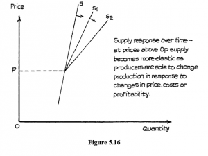
Figure 5.16
SUPPLY, INDIRECT TAXES AND SUBSIDIES
What are Indirect Taxes and Subsidies?
Governments often influence markets through taxes and subsidies.
- An indirect tax is one that is not levied directly on individuals or organisations but is applied at some stage in the production or distribution of goods or services. It therefore affects prices and so is paid indirectly, through price, by consumers and income-earners. For this reason indirect taxes are often referred to as expenditure taxes.
- Direct taxes are those levied directly on income or wealth as it is created and are paid by the income- or wealth-earner to the government. The economic implications of direct taxes are considered later in the course.
At this stage, however, it should be clear to you that anything that influences market price will have consequences for both supply and demand, with the result that the final consequences of a tax may not be what the government intended.
Sometimes, of course, the tax may be imposed with the deliberate intention of influencing supply or demand, but more often it is levied as just another way to raise the revenue that governments imagine they need, and they seek to have as little effect as possible on the production system. In practice, any tax must have an impact, as we shall see.
A subsidy can be seen as a reverse or negative tax. It is a payment to a producer or distributor, so that its effect is to increase supply. To judge the effects of a subsidy, therefore, simply reverse the arguments presented in relation to the tax – but remember, of course, that, in order to pay a subsidy, the government has to have revenue, and its main source of revenue is tax. Generally, then, a subsidy paid to A means that B and C have to be taxed. The harmful effects of the tax may outweigh any beneficial effect of the subsidy.
Effect on Supply
The effect on supply of an indirect tax being imposed is illustrated in Figure 5.17. This shows a supply curve SS, indicating that production can range from 200 units per week at a price of RWF4 to 800 units at a price of RWF10.
Suppose a new tax is imposed at RWF1 per unit. To supply 500 units per week, producers wanted a price of RWF7 per unit. After the imposition of the tax, the producers still want to receive RWF7, but to get this, the price has to rise to RWF8 to include the RWF1 per unit that now has to be paid to the government. Similarly, to keep production at 700 units per week, the price has to rise from RWF9 to RWF10 per unit.
Imposition of the tax thus moves the supply curve to the left (SS to S1S1). The vertical distance between the curves represents the amount of the tax.
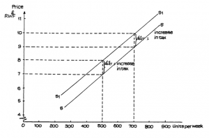
Of course, a subsidy paid to the producer moves the supply curve to the right because the argument is exactly reversed.
In Figure 5.17 the after-tax supply curve S1S1 is parallel to the before-tax curve of SS. This suggests that the tax or tax increase is “flat rate”, i.e. the same at all price levels. In practice indirect taxes such as VAT depend on value and are sometimes known as ad valorem taxes. Usually we would expect the tax to be expressed as a percentage of value or price, and its amount will therefore increase as price rises. In such cases the gap between the two supply curves will increase at the higher prices as illustrated in Figure 5.18.
Although suppliers will be seeking to recover the full amount of any additional expenditure tax from buyers there is no guarantee they will succeed in raising the price sufficiently to achieve this. The extent to which they can recover the tax or have to absorb it in their total costs through the more efficient use of their production resources depends largely on the strength of any price resistance shown by buyers. If buyers cease to buy the product at the increased price suppliers must reconsider their position. The possible consequences of this interaction between suppliers and buyers are examined in Study Unit 6.
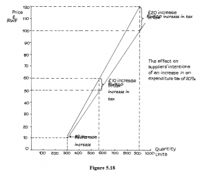
Figure 5.18
The effect on suppliers’ intentions of an increase in an expenditure tax of 20%.