
INTRODUCTION TO PORTFOLIO THEORY
A portfolio is a bundle or a combination of individual assets or securities. Portfolio theory provides a normative approach to investors to make decisions to invest their wealth in assets or securities under risk.1 It is based on the assumption that investors are risk-averse. This implies that investors hold well-diversified portfolios instead of investing their entire wealth in a single or a few assets and they expect high return for high risk and low return for low risk. One important conclusion of the portfolio theory, as we will explain later, is that if the investors hold a well-diversified portfolio of assets, then their concern should be the expected rate of return and risk of the portfolio rather than individual assets and the contribution of individual asset to the portfolio risk. The second assumption of the portfolio theory is that the returns of assets are normally distributed. This means that the mean (the expected value) and variance (or standard deviation) analysis is the foundation of the portfolio decisions. Further, we can extend the portfolio theory to derive a framework for valuing risky assets. This framework is referred to as the capital asset pricing model (CAPM), which we will explain in this chapter.
PORTFOLIO RETURN: TWO-ASSET CASE
The return of a portfolio is equal to the weighted average of the returns of individual assets (or securities) in the portfolio with weights being equal to the proportion of investment value in each asset. Suppose you have an opportunity of investing your wealth in either asset X or asset Y. The possible outcomes of two assets in different states of economy are given in Table 6.1.
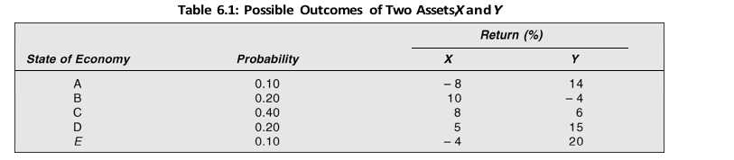
The expected rate of return of X is the sum of the product of outcomes and their respective probability. That is:
E R( x ) ( 8 0.1) (10 0.2) (8 0.4) (5 0.2) ( 4 0.1) 5%
Similarly, the expected rate of return of Y is:
ER( y ) (14 0.1) ( 4 0.2) (6 0.4) (15 0.2) (20 0.1) 8%
We can use the following equation to calculate the expected rate of return of individual asset:
Note that E(Rx) is the expected return on asset X, Ri is ith return and Pi is the probability of ith return.
Suppose you decide to invest 50 per cent of your wealth in X and 50 per cent in Y. What is your expected rate of return on a portfolio consisting of both X and Y ?
The expected rate of return on a portfolio (or simply the portfolio return) is the weighted average of the expected rates of return on assets in the portfolio. In our example, the expected portfolio return is as follows:
![]()
In the case of two-asset portfolio, the expected rate of return is given by the following formula:
Expected return on portfolio = weight of security X × expected return on security X
+ weight of security Y × expected return on security Y
E(Rp) = w × E(Rx) + (1 – w) × E(Ry) (2)
Note that w is the proportion of investment in asset X and (1 – w) is the remaining investment in asset Y.
Given the expected returns of individual assets, the portfolio return depends on the weights (investment proportions) of assets. You may be able to change your expected rate of return on the portfolio by changing your proportionate investment in each asset. How much would you earn if you invested 20 per cent of your wealth in X and the remaining wealth in Y? The portfolio rate of return under this changed mix of wealth in X and Y will be:
ER( p ) 0.2 5 (1 0.2) 8 7.4%
What is the advantage in investing your wealth in both assets X and Y when you could expect highest return of 8 per cent by investing your entire wealth in Y? When you invested your wealth equally in assets X and Y, your expected return is 6.5 per cent. The expected return of Y (8 per cent) is higher than the portfolio return (6.5 per cent). But investing your entire wealth in Y is more risky. Under the unfavourable economic condition, Y may yield a negative return of 4 per cent. The probability of negative return is eliminated when you combine X and Y. You may also note that the expected return of X (5 per cent) is not only less than the portfolio return (6.5 per cent), but it also shows greater fluctuations. We will discuss the concept of risk in greater detail in the following sections.
You may notice that this return is higher than what you will earn if you invested equal amounts in X and Y. The expected return would be 5 per cent if you invested entire wealth in X (i.e., w = 1.0). On the other hand, the expected return would be 8 per cent if the entire wealth were invested in Y (i.e., 1 – w = 1, since w = 0). Your expected return will increase as you shift your wealth from X to Y. Thus, the expected return on portfolio will depend on the percentage of wealth invested in each asset in the portfolio.
Check Your Concepts
- Define the portfolio return.
- How the expected return on a portfolio calculated?
PORTFOLIO RISK: TWO-ASSET CASE
We have seen in the previous section that returns on individual assets fluctuate more than the portfolio return. Thus, individual assets are more risky than the portfolio. How is the risk of a portfolio measured? As discussed in the previous chapter, risk of individual assets is measured by their variance or standard deviation. We can use variance or standard deviation to measure the risk of the portfolio of assets as well. Why is a portfolio less risky than individual assets? Let us consider an example.
Suppose you have two investment opportunities A and B as shown in Table 6.2.
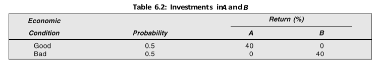
Assuming that the investor invests in both the assets equally, the expected rate of return, variance and standard deviation of A are:
E R( A ) 0.5 40 0.5 0 20%
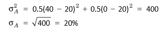
Here A represents the standard deviation of assets A, A2 is the variance of asset A and E(RA) is the estimated rate of returns. Note that variance is the square of standard deviation.
Similarly, the expected rate of return, variance and standard deviation of B are:
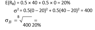
Both investments A and B have the same expected rate of return (20 per cent) and same variance (400) and standard deviation (20 per cent). Thus, they are equally profitable and equally risky. How does combining investments A and B help an investor? If a portfolio consisting of equal amount of A and B were constructed, the portfolio return would be:
E R( P ) 0.5 20 0.5 20 20%
This return is the same as the expected return from individual securities, but without any risk. Why? If the economic conditions are good, then A would yield 40 per cent return and B zero and the portfolio return will be:
E R( P ) 0.5 40 0.5 0 20%
When economic conditions are bad, then A’s return will be zero and B’s 40 per cent and the portfolio return would still remain the same:
E R( P ) 0.5 0 0.5 40 20%
Thus, by investing equal amounts in A and B, rather than the entire amount only in A or B, the investor is able to eliminate the risk altogether. She is assured of a return of 20 per cent with a zero standard deviation.
It is not always possible to entirely reduce the risk. It may be difficult in practice to find two assets whose returns move completely in opposite directions like in the above example of securities A and B. It needs emphasis to state that the risk of portfolio would be less than the risk of individual securities, and that the risk of a security should be judged by its contribution to the portfolio risk.
Measuring Portfolio Risk for Two Assets
Like in the case of individual assets, the risk of a portfolio could be measured in terms of its variance or standard deviation. As stated earlier, the portfolio return is the weighted average of returns on individual assets. Is the portfolio variance or standard deviation a weighted average of the individual assets’ variances or standard deviations? It is not. The portfolio variance or standard deviation depends on the co-movement of returns on two assets.
Covariance
When we consider two assets, we are concerned with the co-movement of the assets. Covariance of returns on two assets measures their co-movement. How is covariance calculated?
Three steps are involved in the calculation of covariance between two assets:
Determining the expected returns on assets.
Determining the deviation of possible returns from the expected return for each asset. Determining the sum of the product of each deviation of returns of two assets and respective probability.
Let us consider the data of securities of X and Y given in Table 6.3. The expected return on security X is:
E R( x ) (0.1 8) (0.2 10) (0.4 8) (0.2 5) (0.1 4) 5%
Security Y’s expected return is:
ER( y ) ![]()
If the equal amount is invested in X and Y, the expected return on the portfolio is:
ER( p) ![]()
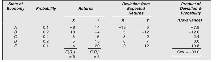
The covariance of returns of securities X and Y is –33.0. The formula for calculating covariance of returns of the two securities X and Y is as follows:
n
Covxy [R ER R ER Px ( x )][ y ( y)] i (3)
i 1
Note that Covxy is the covariance of returns on securities X and Y, Rx and Ry returns on securities X and Y respectively, E(Rx) and E(Ry) expected returns of X and Y respectively and Pi probability of occurrence of the state of economy i. Using Equation (3), the covariance between the returns of securities X and Y can be calculated as shown below:
Covxy = 0.1(–8 – 5)(14 – 8) + 0.2(10 – 5)(–4 – 8) + 0.4(8 – 5)(6 – 8)
+ 0.2(5 – 5)(15 – 8) + 0.1(–4 – 5)(20 – 8)
= –7.8 – 12 – 2.4 + 0 – 10.8 = –33.0
What is the relationship between the returns of securities X and Y? There are following possibilities:
Positive covariance X ’s and Y ’s returns could be above their average returns at the same time. Alternatively, X ’s and Y ’s returns could be below their average returns at the same time. In either situation, this implies positive relation between two returns. The covariance would be positive.
Negative covariance X ’s returns could be above its average return while Y ’s return could be below its average return and vice versa. This denotes a negative relationship between returns of X and Y. The covariance would be negative.
Zero covariance Returns on X and Y could show no pattern; that is, there is no relationship. In this situation, covariance would be zero. In reality, covariance may be non-zero due to randomness and the negative and positive terms may not cancel out each other.
In our example covariance between returns on X and Y is negative, that is, –33.0. This is akin to the second situation above; that is, two returns are negatively related. What does the number –33.0 imply? As in the case of variance, covariance also uses squared deviations and therefore, the number cannot be explained. We can, however, compute the correlation to measure the relationship between two returns.
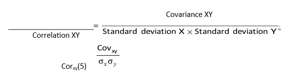
Correlation
Covariance XY Standard deviation X Standard deviation Y Correlation XY (4) Covxy x yCorxy
How can we find relationship between two variables? Correlation is a measure of the linear relationship between two variables (say, returns of two securities, X and Y in our case). It may be observed from Equation (3) that covariance of returns of securities X and Y is a measure of both variability of returns of securities and their association. Thus, the formula for covariance of returns on X and Y can also be expressed as follows:
Note that x and y are standard deviations of returns for securities X and Y and Corxy is the correlation between returns of X and Y. From Equation (4), we can determine the correlation by dividing covariance by the standard deviations of returns on securities X and Y:
The value of correlation, called the correlation coefficient, could be positive, negative or zero. It depends on the sign of covariance since standard deviations are always positive numbers. The correlation coefficient always ranges between –1.0 and +1.0. A correlation coefficient of +1.0 implies a perfectly positive correlation while a correlation coefficient of –1.0 indicates a perfectly negative correlation. The correlation between the two variables will be zero (or not different from zero) if they are not at all related to each other. In a number of situations, returns of any two securities maybe weakly correlated (negatively or positively).
Let us calculate correlation by using data given in Table 6.3. The covariance is –33.0. We need standard deviations of X and Y to compute the correlation. The standard deviation of securities X and Y are as follows:
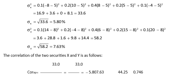
Securities X and Y are negatively correlated. The correlation coefficient of –0.746 indicates a high negative relationship. If an investor invests her wealth in both instead any one of them, she can reduce the risk. How?
Variance and Standard Deviation of a Two-Asset Portfolio
We know now that the variance of a two-asset portfolio is not the weighted average of the variances of assets since they co-vary as well. The variance of two-security portfolio is given by the following equation:
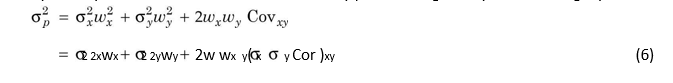
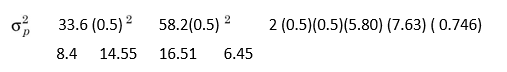
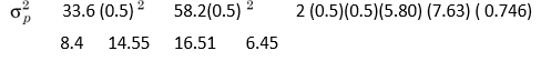
Applying Equation (6), the variance of portfolio of X and Y will be as follows:
It may be noticed from Equation (6) that the variance of a portfolio includes the proportionate variances of the individual securities and the covariance of the securities. The covariance depends on the correlation between the securities in the portfolio. The risk of the portfolio would be less than the weighted average risk of the securities for low or negative correlation.
The standard deviation of two-asset portfolio is the square root of variance:
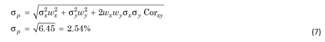
What does the portfolio standard deviation of 2.54 per cent mean? The implication is the same as in the case of the standard deviation of an individual asset (security). The expected return on the portfolio is 6.5 per cent, and it could vary between 3.96 per cent [i.e., 6.5 – 2.54] and 9.04 per cent [i.e., 6.5 + 2.54] within one standard deviation from the mean. There is about 68 per cent probability that the portfolio return would range between 3.96 per cent and 9.04 per cent if we assume that the portfolio return is normally distributed.
Minimum Variance Portfolio
What is the best combination of two securities so that the portfolio variance is minimum? The minimum variance portfolio is also called the optimum portfolio. However, investors do not necessarily strive for the minimum variance portfolio. A risk-averse investor will have a tradeoff between risk and return. Her choice of a particular portfolio will depend on her risk preference.
We can use the following general formula for estimating optimum weights of two securities X and Y so that the portfolio variance is minimum:
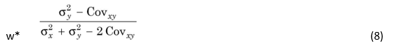
where w* is the optimum proportion of investment or weight in security X. Investment in Y will be: 1 – w*. In the example above, we find that w* is:
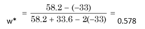
Thus the weight of Y will be: 1 – 0.578 = 0.422.
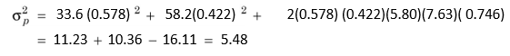
The portfolio variance (with 57.8 per cent of investment in X and 42.2 per cent in Y) is:
The standard deviation is:
![]()
Portfolio Risk Depends on Correlation between Assets
Any other combination of X and Y will yield a higher variance or standard deviation.
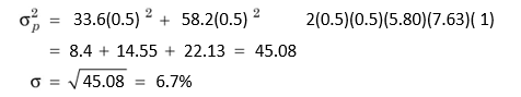
We emphasize once again that the portfolio standard deviation is not the weighted average of the standard deviations of the individual securities. In our example above, the standard deviation of portfolio of X and Y is 2.54 per cent. Let us see how much is the weighted standard deviation of the individual securities:
Weighted standard deviation of individual securities
= 5.8 × 0.5 + 7.63 × 0.5 = 6.7%
Thus, the standard deviation of portfolio of X and Y is considerably lower than the weighted standard deviation of these individual securities. This example shows that investing wealth in more than one security reduces portfolio risk. This is attributed to diversification effect. However, the extent of the benefits of portfolio diversification depends on the correlation between returns on securities. In our example, returns on securities X and Y are negatively correlated and the correlation coefficient is –0.746. This has caused significant reduction in the portfolio risk. Would there be diversification benefit (that is, risk reduction) if the correlation were positive? Let us assume that correlation coefficient in our example is +0.25. How much is the portfolio standard deviation? (Using Eq. 7) It is 5.34, as shown below:
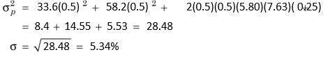
The portfolio risk (s = 5.34%) is still lower than the weighted average standard deviation of individual securities (s = 6.7%). If the returns of securities X and Y are positively and perfectly correlated (with the correlation coefficient of 1), then the portfolio standard deviation is as follows:
When correlation coefficient of the returns on individual securities is perfectly positive (i.e., Cor = 1.0), then there is no advantage of diversification. The weighted standard deviation of returns on individual securities is equal to the standard deviation of the portfolio. We may therefore conclude that diversification always reduces risk provided the correlation coefficient is less than 1.
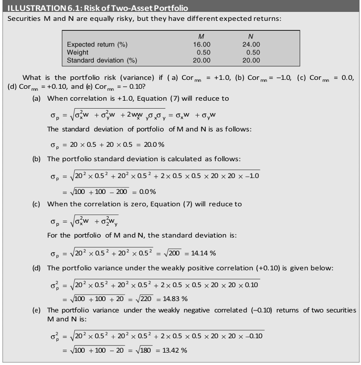
It may be observed in the above example that a total reduction of risk is possible if the returns of the two securities are perfectly negatively correlated, though, such a perfect negative correlation will not generally be found in practice. Securities do have a tendency of moving together to some extent, and therefore, risk may not be totally eliminated.
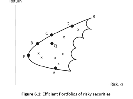
Efficient Portfolio
An investor can combine securities or assets to form several portfolios. However, all portfolios may not be efficient in terms of risk-return relationship. An efficient portfolio2 is one that has the highest expected returns for a given level of risk. The efficient frontier is the frontier formed by the set of efficient portfolios. In Figure 6.1, the curve starting from portfolio P, which is the minimum variance portfolio, and extending to the portfolio R is the efficient frontier. All portfolios on the efficient frontier are efficient portfolios since higher risk obtains higher returns. All other portfolios, which lie outside the efficient frontier, are inefficient portfolios. For example, portfolio Q has same return as portfolio B but it has higher risk. Similarly, portfolio C has higher return than portfolio Q with same amount of risk. Q is an inefficient portfolio. Portfolios B and C are efficient portfolios—portfolio B has low risk and low return, while portfolio C has high risk and high return. B dominates C. The choice of the portfolio will depend on the investor’s risk-return preference.
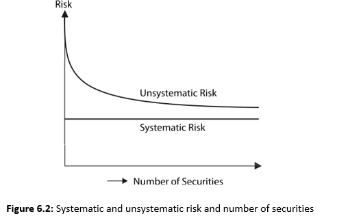
RISK DIVERSIFICATION
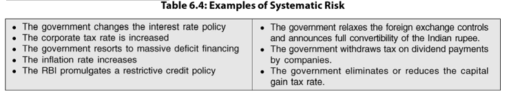
Can diversification reduce all risk of securities? When more and more securities are included in a portfolio, the risk of individual securities in the portfolio is reduced. This risk totally vanishes when the number of securities is very large. But the risk represented by covariance remains. Thus, risk has two parts: diversifiable (unsystematic) and non-diversifiable (systematic).3
Systematic Risk
Non-diversifiable risk is called systematic risk. Systematic risk arises on account of the economy-wide uncertainties and the tendency of individual securities to move together with changes in the market. This part of risk cannot be reduced through diversification. It is also known as market risk. Investors are exposed to market risk even when they hold welldiversified portfolios of securities.4 The examples of systematic or market risk are given in Table 6.4.
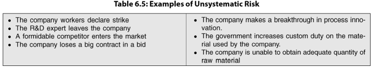
Unsystematic Risk
Diversifiable risk is called unsystematic risk. Unsystematic risk arises from the unique uncertainties of individual securities. It is also called unique risk. These uncertainties are diversifiable if a large numbers of securities are combined to form well-diversified portfolios. Uncertainties of individual securities in a portfolio cancel out each other. Thus unsystematic risk can be totally reduced through diversification. Table 6.5 contains examples of unsystematic risks.
Total Risk
Total risk of an individual security is the variance (or standard deviation) of its return. It consists of two parts:
Total risk of a security = Systematic risk + Unsystematic risk (14)
Systematic risk is attributable to macroeconomic factors. An investor has to suffer the systematic risk, as it cannot be diversified away. The unsystematic risk is firm specific. Thus, Equation (14) can be written as:
Total risk = variance attributable to macroeconomic factors
+ (residual) variance attributable to firm-specific factors (15)
Total risk is not relevant for an investor who holds a diversified portfolio. The systematic risk cannot be diversified, and therefore, she will expect a compensation for bearing this risk. She will be more concerned about that portion of the risk of individual securities that she cannot diversify.
Figure 6.2 shows that unsystematic risk can be reduced as more and more securities are added to a portfolio. How many securities should be held by an investor to eliminate unsystematic risk? In USA, it has been found that holding about 15 shares can eliminate unsystematic risk.5 In the Indian context, a portfolio of 40 shares can almost totally eliminate such a risk.6 Diversification is not able to reduce the systematic risk. Thus, the source of risk for an investor who holds a well-diversified portfolio is that the market will swing due to economic activities affecting the investor’s portfolio. Typically, the diversified portfolios move with the market. The most common well-diversified portfolios in India include the share indices of the Bombay Stock Exchange and the National Stock Exchange. In a study in USA, it has been found that market risk contributes about 50 per cent variation in the price of a share.7 Thus diversification may be able to eliminate only half of the total risk (viz., unsystematic risk). How can we measure systematic (i.e., market) risk? What is the relationship between risk and return?
COMBINING A RISK-FREE ASSET AND A RISKY ASSET
In the preceding sections, we have discussed the risk-return implications of holding risky securities. What happens to the choices of investors in the market if they could combine a risk-free security with a single or multiple risky securities? If investors could borrow and lend at the risk-free rate of interest, how would the portfolio opportunity set be shaped and how could securities be valued in the market?
A risk-free asset or security has a zero variance or standard deviation and has no risk of default. The government treasury bills or bonds are approximate examples of the risk-free security as they have no risk of default and have very low standard deviation.
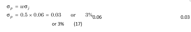
What happens to return and risk when we combine a risk-free and a risky asset? Let us assume that an investor holds a risk-free security f, of which he has an expected return of 5 per cent and a risky security j, with an expected return of 15 per cent and a standard deviation of 6 per cent. What is the portfolio return and risk if the investor holds these securities in equal proportion? The portfolio return is:
E R( p) wER( j ) (1 w R) f
0.5 0.15 (1 0.5)0.05
0.075 0.025 0.10 or 10% (16)
Since the risk-free security has zero standard deviation, the covariance between the risk-free security and risky security is also zero. The portfolio risk is simply given as the product of the standard deviation of the risky security and its weight. Thus
Borrowing and Lending
The investor can invest all her wealth in the risk-free security or the risky-security. She may even borrow funds at the risk-free rate of interest and invest more than 100 per cent of her wealth in the risky security. Alternatively, she may invest less than 100 per cent in the risky security and lend the remaining funds at the risk-free rate of interest. Under different combinations of the risky security and the risk-free security, with borrowing and lending at the risk-free rate of interest, the expected return and risk could be calculated as shown in Table 6.6.
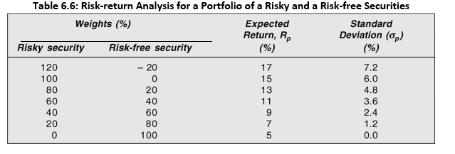
Figure 6.3 illustrates the risk-return relationship for various combinations of a risk-free security and a risky security, and the resulting portfolio opportunity set. Point B represents 100 per cent investment in the risky security expected to yield 15 per cent return and 6 per cent standard deviation. The investor can borrow at the risk-free rate and invest in the risky security. Point C (to the right of Point B) shows 120 per cent investment in the risky security after borrowing at the risk-free rate of interest and the investor can expect to earn a return of 17 per cent with a higher risk, viz., a standard deviation of 7.2 per cent. A risk-averse investor may not invest her entire wealth in the risky security, and may like to lend a part of her wealth at the risk-free rate of interest. Point A (to the left of Point B) illustrates this behaviour. At Point A the investor invests 60 per cent of her wealth in the risky security and lends the remaining amount at 5 per cent risk-free rate of interest. She can expect to earn a return of 11 per cent with a standard deviation of 3.6 per cent. A very conservative investor may lend her entire wealth at the risk-free rate of interest. Point Rf shows that when the
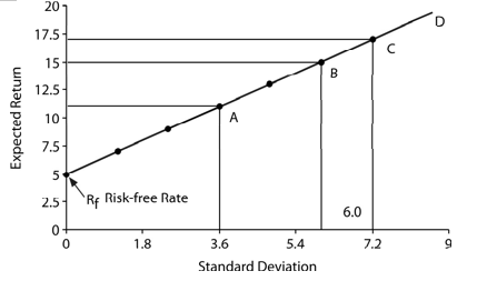
Figure 6.3: Risk-return relationship for portfolio of risky and risk-free securities
investor lends her entire wealth, she could earn 5 per cent return with zero risk. Theoretically, it is possible that an investor may borrow and invest (lend) more than 100 per cent at the risk-free rate of interest. No investor will do this in practice since his or her return will be less for equal or more risk than for a lending-borrowing combination along the line Rf D. Thus line Rf D illustrates the portfolio opportunity set for the possible combinations of a risk-free security and a risky security.
Check Your Concepts
- Define a risk-free asset. Give an example.
- What is the risk of a portfolio consisting of a risk-free asset and a risky asset?
- How does borrowing and lending help in determining opportunity set of a risk-free asset andrisky asset?
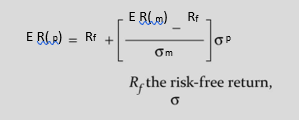
CAPITAL ASSET PRICING MODEL (CAPM)
The capital asset pricing model (CAPM) is a model that provides a framework to determine the required rate of return on an asset and indicates the relationship between return and risk of the asset.8 The required rate of return specified by CAPM helps in valuing an asset. One can also compare the expected (estimated) rate of return on an asset with its required rate of return and determine whether the asset is fairly valued. As we will explain in this section, under CAPM, the security market line (SML) exemplifies the relationship between an asset’s risk and its required rate of return.
We have so far discussed the principles of portfolio choices as made by investors. We also considered the significance of the risk-free asset in portfolio decisions. In the presence of the risk-free asset, the capital market line (CML) is the relevant efficient frontier, and all investors would choose to remain on the CML. This implies that the relevant measure of an asset’s risk is its covariance with the market portfolio of risky assets. How do we determine the required rate of return on a risky asset? How is an asset’s risk related to its required rate of return?
Assumptions of CAPM
The capital asset pricing model, or CAPM, envisages the relationship between risk and the expected rate of return on a risky security. It provides a framework to price individual securities and determine the required rate of return for individual securities. It is based on a number of simplifying assumptions. The most important assumptions are:9
Market efficiency The capital market efficiency implies that share prices reflect all available information. Also, individual investors are not able to affect the prices of securities. This means that there are large numbers of investors holding a small amount of wealth.
Risk aversion and mean-variance optimization Investors are risk-averse. They evaluate a security’s return and risk in terms of the expected return and variance or standard deviation, respectively. They prefer the highest expected returns for a given level of risk. This implies that investors are mean-variance optimizers and they form efficient portfolios.
Homogeneous expectations All investors have the same expectations about the expected returns and risks of securities.
Single time period All investors’ decisions are based on a single time period. Risk-free rate All investors can lend and borrow at a risk-free rate of interest. They form portfolios from publicly traded securities like shares and bonds.
Capital Market Line (CML)
Under CAPM, all investors are assumed to have homogeneous expectations, and their borrowing and lending rate is the same. They all will hold the same risky portfolio. If so, this portfolio, in equibrium, is referred to as the market portfolio. Market portfolio is that portfolio that comprises all risky assets. The proportion of each asset is equal to its value to the total value of all risky assets. The efficient frontier, comparing market portfolio with lending and borrowing is shown in Figure 6.4.
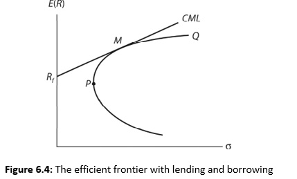
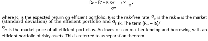
All investors will combine market portfolio and the risk-free security. The straight line formed by joining Rf through M to other efficient portfolios is called the capital market line (CML). Thus all efficient portfolios will lie on the capital market line. What is the price of the risk? The equation for the capital market line is:
Characteristic Line
We know from the earlier discussion that risk has two parts: unsystematic risk, which can be eliminated through diversification, and systematic risk, which cannot be reduced. Since unsystematic risk can be mostly eliminated without any cost, there is no price paid for it. Therefore, it will have no influence on the return of individual securities. Market will pay premium only for systematic risk since it is non-diversifiable. How can we measure the risk of individual securities and their risk-adjusted required rates of return? Let us consider an example.
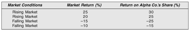
The following table gives probable rates of return on a market portfolio (represented by an index like the sensex) and on Alpha Company’s share. There are two possibilities with regard to market conditions, either the market will rise or it will fall. Under each market condition, there are two equally likely outcomes for both the market portfolio and Alpha.
Let us examine the behaviour of the market return and return on Alpha’s share. The expected return for the market and Alpha are as follows:
Rising market:
Expected market return = 0.5 × 25 + 0.5 × 20 = 22.5%
Expected Alpha return = 0.5 × 30 + 0.5 × 25 = 27.5% Falling market:
Expected Alpha return = 0.5 × –25 + 0.5 × –15 = –20.0%
Expected market return = 0.5 × –15 + 0.5 × –10 = –12.5%
The market return in the rising market is 22.5 per cent and it is –12.5 per cent in the falling market. This means that the market return is 35 per cent higher in the rising market when compared to the market return in the falling market. In case of Alpha, the return in the rising market is 47.5 per cent higher compared to the market return in the falling market. How sensitive is Alpha’s return in relation to the market return? Alpha’s return increases by 47.5 per cent compared to 35 per cent increase in the market return in the rising market conditions. Alternatively, Alpha’s return declines by 47.5 per cent compared to 35 per cent decrease in the market return in the falling market conditions. Thus the sensitivity of the Alpha’s return vis-à-vis the market return is: 47.5%/35% = 1.36. We can refer to this number as the sensitivity coefficient. The sensitivity coefficient of 1.36 implies that for a unit change (increase or decrease) in the market return, Alpha’s return will change by 1.36 times. The sensitivity of the Alpha’s return vis-á-vis the market return reflects its risk. The sensitivity coefficient is called beta.
We plot the combinations of four possible returns of Alpha and market in Figure 6.5. They are shown as four points. The combinations of the expected returns points (22.5%, 27.5% and –12.5%, –20%) are also shown in the figure. We join these two points to form a line. This line is called the characteristic line. The slope of the characteristic line is the sensitivity coefficient, which, as stated earlier, is referred to as beta.
Security Market Line (SML)
Under CAPM, the risk of an individual risky security is defined as the volatility of the security’s return vis-á-vis the return of the market portfolio. This risk of an individual risky security is
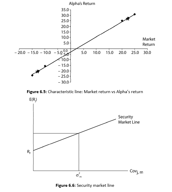
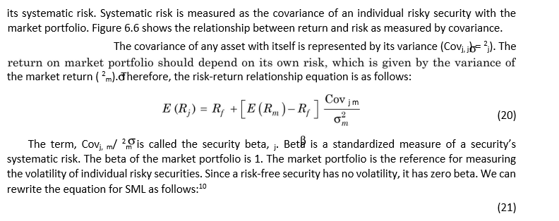
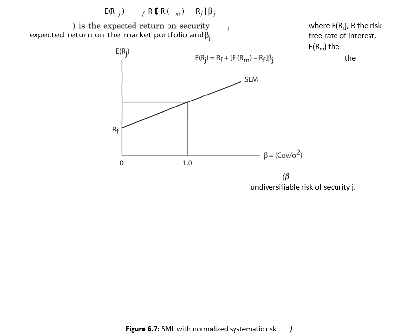
Figure 6.7 illustrates SML with normalized systematic risk as measured by beta. Figure 6.6 and Equation (21) show that the required rate of return on a security is equal to a risk-free rate plus the risk-premium for the risky security. The risk-premium on a risky security equals the market risk premium, that is, the difference between the expected market return and the risk-free rate. Since the market risk premium is same for all securities, the total
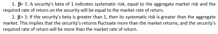
 < 1: On the other hand, a security’s beta of less than 1 means that the security’s risk is lower than the aggregate market risk. This implies that the security’s returns are less sensitive to the changes in the market returns. The security’s required rate of return will be less than the market rate of return.
Can a security’s beta be negative? Theoretically, beta can be negative. A security with negative beta would earn less than the risk-free rate of return
ILLUSTRATION 6.2: Required Rate of Return Calculation
The risk-free rate of return is 8 per cent and the market rate of return is 17 per cent. Betas for four shares, P, Q, R and S are, respectively, 0.60, 1.00, 1.20 and –0.20. What are the required rates of return on these four shares? We can use Equation (21) to calculate the required rates of return.
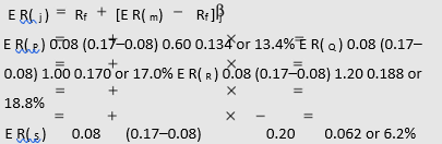
Q with beta of 1.00 has a return equal to the market return. P has beta lower than 1.00, therefore its required rate of return is lower than the market return. R has a return greater than the market return since its beta is greater than 1.00. S has a return lower than the risk-free rate since it has a negative beta.
IMPLICATIONS AND RELEVANCE OF CAPM
CAPM is based on a number of assumptions. Given those assumptions, it provides a logical basis for measuring risk and linking risk and return.
Implications
CAPM has the following implications:
Investors will always combine a risk-free asset with a market portfolio of risky assets. They will invest in risky assets in proportion to their market value.
Investors will be compensated only for that risk which they cannot diversify. This is the market-related (systematic) risk. Beta, which is a ratio of the covariance between the asset returns and the market returns divided by the market variance, is the most appropriate measure of an asset’s risk.
Investors can expect returns from their investment according to the risk. This implies a linear relationship between the asset’s expected return and its beta.
The concepts of risk and return as developed under CAPM have intuitive appeal and they are quite simple to understand. Financial managers use these concepts in a number of financial decision making, such as valuation of securities, cost of capital measurement, investment risk analysis, etc. However, in spite of its intuitive appeal and simplicity, CAPM suffers from a number of practical problems.
Limitations
CAPM has the following limitations:
It is based on unrealistic assumptions
It is difficult to test the validity of CAPM
Betas do not remain stable over time
Unrealistic Assumptions
CAPM is based on a number of assumptions that are far from the reality. For example, it is very difficult to find a risk-free security. A short-term, highly liquid government security is considered to be a risk-free security. It is unlikely that the government will default, but inflation causes uncertainty about the real rate of return. The assumption of the equality of the lending and borrowing rates is also not correct. In practice, these rates differ. Further, investors may not hold highly diversified portfolios, or the market indices may not be well diversified. Under these circumstances, CAPM may not accurately explain the investment behaviour of investors and the beta may fail to capture the risk of investment.
Testing CAPM
Most of the assumptions of CAPM may not be very critical for its practical validity. What we need to know, therefore, is the empirical validity of CAPM. We need to establish that beta is able to measure the risk of a security and that there is a significant correlation between the beta and the expected return. The empirical results have given mixed results. The earlier tests showed that there was a positive relation between returns and betas. However, the relationship was not as strong as predicted by CAPM. Further, these results revealed that returns were also related to other measures of risk, including the firm-specific risk. In subsequent research, some studies did not find any relationship between betas and returns.
On the other hand, other factors such as size and the market value and book value ratios were found as significantly related to returns.11
All empirical studies testing CAPM have a conceptual problem. CAPM is an ex ante model; that is, we need data on expected prices to test CAPM. Unfortunately, in practice, the researchers have to work with the actual past (ex post) data. Thus, this will introduce bias in the empirical results.
Stability of Beta
Beta is a measure of a security’s future risk. But investors do not have future data to estimate beta. What they have is past data about the share prices and the market portfolio. Thus, they can only estimate beta based on historical data. Investors can use historical beta as the measure of future risk only if it is stable over time. Research has shown that the betas of individual securities are not stable over time. This implies that historical betas are poor indicators of the future risk of securities.
Relevance of CAPM
CAPM is a useful device for understanding the risk-return relationship in spite of its limitations. It provides a logical and quantitative approach for estimating risk. It is better than many alternative subjective methods of determining risk and risk premium. One major problem in the use of CAPM is that many times the risk of an asset is not captured by beta alone.
Check Your Concepts
- What is capital asset pricing model (CAPM)?
- What are the assumptions of CAPM?
- What is beta? How is it calculated?
Define the characteristic line.
- Define security market line (SLM).
Summary
Generally, investors in practice hold multiple securities. Combinations of multiple securities are called portfolios.
The expected return on a portfolio is the sum of the returns on individual securities multiplied by their respective weights (proportionate investment). That is, it is a weighted average rate of return. In the case of a twosecurity portfolio, the portfolio return is given by the following equation:

The portfolio risk is not a weighted average risk. Securities included in a portfolio are associated with each other. Therefore, the portfolio risk also accounts for the covariance between the returns of securities. Covariance is the product of the standard deviations of individual securities and their correlation coefficient.
As the number of securities in the portfolio increases, the portfolio variance approaches the average covariance. Thus, diversification helps in reducing the risk.
The investment or portfolio opportunity set represents all possible combinations of risk and return, resulting from portfolios, formed by varying proportions of individual securities. It presents the investor with the riskreturn tradeoff.
For a given risk, an investor would prefer a portfolio with higher expected rate of return. Similarly, when the expected returns are same, she would prefer a portfolio with lower risk. The choice between high riskhigh return or low risklow return portfolios will depend on the investor’s risk preference. This is refereed to as the meanvariance criterion.
An efficient portfolio is one that has the highest expected returns for a given level of risk. The efficient frontier is the frontier formed by the set of efficient portfolios.
The optimum risky portfolio is the market portfolio of all risky assets where each asset is held in proportion of its market value. It is the best portfolio since it dominates all other portfolios. An investor can thus mix her borrowing and lending with the best portfolio according to her risk preferences. She can invest in two separate investments—a risk free asset and a portfolio of risky securities. This is known as the separation theorem.
Risk has two parts: unsystematic risk and systematic risk.
Unsystematic risk can be eliminated through diversification. It is a risk unique to a specific security. When individual securities are combined, their unique risks cancel out.
Systematic risk cannot be eliminated through diversification. It is a marketrelated risk. It arises because individual securities move with the changes in the market.
Investors are riskaverse. They will take risk only if they are compensated for the risk, which they bear. Since systematic risk cannot be eliminated through diversification, they will be compensated for assuming the systematic risk.
The market prices the risky securities in a manner that they yield higher expected returns than the riskfree securities. The riskaverse investors can be induced to hold risky securities when they are offered a risk premium. The capital market line (CML) defines this relationship. The equation for CML is:
where E (Rp) is the portfolio return
, E (Rm) the return on market portfolio, m the standard deviation of market portfolio and p the standard deviation of the portfolio.
The model explaining the riskreturn relationship is called the capital asset pricing model (CAPM). It provides that in a wellfunctioning capital market, the risk premium varies in direct proportion to risk.
CAPM provides a measure of risk and a method of estimating the market’s riskreturn line. The market (systematic) risk of a security is measured in terms of its sensitivity to the market movements. This sensitivity is referred to as the security’s beta.
Review Questions
- What is a portfolio? How are the portfolio return and risk calculated for a two-security portfolio?
- Does diversification reduce the risk of investment? Explain with an example.
- Define systematic and unsystematic risks. Give examples of both.
- What is the capital asset pricing model? Explain its assumptions and implications.
- Explain the security market line (SML) with the help of a figure.
Quiz Exercises
- You hold your investment in two assets—X and Y—in proportions of 60 per cent and 40 per cent, respectively. You expect a return of 12 per cent from X and 14 per cent from Y. What is your return from the portfolio of X and Y?
- Your return on HUL’s share may either yield a return of 24 per cent with 75 per cent chance or7 per cent with 25 per cent chance. What is your expected return?
- You have investments in assets A and B. You have equal chances of earning either 24 per cent or 12 per cent or 6 per cent on A and either 33 per cent or 9 per cent or –6 per cent on B under three different economic situations. Calculate (i) expected return and variance of the expected return for A and B; (ii) covariance of the expected returns of A and B.
- The correlation between the returns of assets L and M is 0.60. The standard deviations of returns of L and M are respectively 8 and 12. Calculate covariance of returns of L and M.
- The covariance between the returns of assets P and Q is –33. The standard deviations of returns of P and Q are respectively 5.8 and 7.6. Calculate correlation of returns of P and Q.
- Security C has expected return of 20 per cent and standard deviation of 25 per cent. On the other hand, security D has expected return of 24 per cent and standard deviation of 25 per cent. Both securities have equal weights in the portfolio. Calculate the portfolio variance if the correlation is (i) 0.00; (ii) 0.20; (iii) 0.80 and (iv) –0.20. What inferences do you make from the calculations?
- The risk-free rate of return is 6 per cent. The market rate of return is 12 per cent with a standarddeviation of 8 per cent. If you desire to earn a rate of return of 10 per cent, in what proportion should you hold market portfolio and the risk-free asset?
- The variance of market returns is 0.05 and the covariance between market returns and returnson X’s shares is 0.084. What is X’s beta?