
INTRODUCTION
We’ve seen how the correlation coefficient measures the degree of relationship between two variates.With perfect correlation (r = +1.0 or r = -1.0), the points of the scatter diagram all lie exactly on a straightline. It is sometimes the case that two variates are perfectly related in some way such that the points would lie exactly on a line, but not a straight line. In such a case r would not be 1.0. This is a most important point to bear in mind when you have calculated a correlation coefficient; the value may be small, but the reason may be that the correlation exists in some form other than a straight line.
The correlation coefficient tells us the extent to which the two variates are linearly related, but it does not tell us how to find the particular straight line which represents the relationship. The problem of determining which straight line best fits the points of a particular scatter diagram comes under the heading of LINEAR REGRESSION analysis.
Remember that a straight-line graph can always be used to represent an equation of the form y = mx+ c. In such an equation, y and x are the variables while m and c are the constants. Figure 8.1 shows a few examples of straight-line graphs for different values of m and c. Note the following important features of these linear graphs:
− The value of c is always the value of y corresponding to x = 0.
− The value of m represents the gradient or slope of the line. It tells us the number of units change in y per unit change in x. Larger values of m mean steeper slopes.
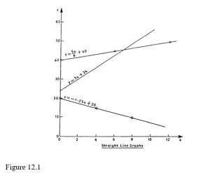
Negative values of the gradient, m, mean that the line slopes downwards to the right; positive values of the gradient, m, mean that the line slopes upwards to the right.
So long as the equation linking the variables y and x is of the form y = mx + c, it is always possible to represent it graphically by a straight line. Likewise, if the graph of the relationship between y and x is a straight line, then it is always possible to express that relationship as an equation of the form y=mx+c.
Often in regression work the letters a and b are used instead of c and m, i.e. the regression line is written as y = a + bx. You should be prepared to meet both forms.
If the graph relating y and x is NOT a straight line, then a more complicated equation would be needed. Conversely, if the equation is NOT of the form y = mx + c (if, for example, it contains terms like x2 or log x) then its graph would be a curve, not a straight line.
REGRESSION LINES
Nature of Regression Lines
When we have a scatter diagram whose points suggest a straight-line relationship (though not an exact one), and a correlation coefficient which supports the suggestion (say, r equal to more than about 0.4 or 0.5), we interpret this by saying that there is a linear relationship between the two variables but there are other factors (including errors of measurement and observation) which operate to give us a scatter of points around the line instead of exactly on it.
In order to determine the relationship between y and x, we need to know what straight line to draw through the collection of points on the scatter diagram. It will not go through all the points, but will lie somewhere in the midst of the collection of points and it will slope in the direction suggested by the points. Such a line is called a REGRESSION LINE.
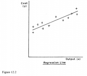
In Figure 12.2 x is the monthly output of a factory and y is the total monthly costs of the factory; the scatter diagram is based on last year’s records. The line which we draw through the points is obviously the one which we think best fits the situation, and statisticians often refer to regression lines as lines of best fit. Our problem is how to draw the best line.
Graphical Method
It can be proved mathematically (but you don’t need to know how!) that the regression line must pass through the point representing the arithmetic means of the two variables. The graphical method makes use of this fact, and the procedure is as follows:
- Calculate the means and of the two variables.
- Plot the point corresponding to this pair of values on the scatter diagram.
- Using a ruler, draw a straight line through the point you have just plotted and lying, as evenly as you can judge, among the other points on the diagram.
In Figure 12.3 the above procedure was followed using the data from the section on the correlation coefficient in the previous study unit. If someone else (you, for example) were to do it, you might well get a line of a slightly different slope, but it would still go through the point of the means (marked +).
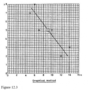
Quite obviously, this method is not exact (no graphical methods are) but it is often sufficient for practical purposes. The stronger the correlation, the more reliable this method is, and with perfect correlation there will be little or no error involved.
Mathematical Method
A more exact method of determining the regression line is to find mathematically the values of the constants m and c in the question y = mx + c, and this can be done very easily. This method is called the least squares method, as the line we obtain is that which minimises the sum of the squares of the vertical deviations of the points from the line
The regression line which we have drawn, and the equation which we have determined, represent the regression of y upon x. We could, by interchanging x and y, have obtained the regression of x on y. This would produce a different line and a different equation. This latter line is shown in Figure 8.4 by a broken line. The question naturally arises, “Which regression line should be used?”. The statistician arrives at the answer by some fairly complicated reasoning but, for our purposes, the answer may be summed up as follows:
- Always use the regression of y on x. That is, use the method described in detail above, putting y on the vertical axis and x on the horizontal
- If you intend to use the regression line to predict one thing from another, then the thing you want to predict is treated as y; the other thing is x. For example, if you wish to use the regression line (or its equation) to predict costs from specified outputs, then the outputs will be the x and the costs will be the y.
- If the regression is not to be used for prediction, then the x should be the variate whose value is known more reliably.
CONNECTION BETWEEN CORRELATION AND REGRESSION
The degree of correlation between two variables is a good guide to the likely accuracy of the estimates made from the regression equation. If the correlation is high then the estimates are likely to be reasonably accurate, and if the correlation is low then the estimates will be poor as the unexplained variation is then high.
You must remember that both the regression equations and the correlation coefficient are calculated from the same data, so both of them must be used with caution when estimates are predicted for values outside the range of the observations, i.e. when values are predicted by extrapolation or the correlation coefficient is assumed to remain constant under these conditions. Also remember that the values calculated for both correlation and regression are influenced by the number of pairs of observations used. So results obtained from a large sample are more reliable than those from a small sample.
Questions on correlation and regression are frequently set in examinations and they are also in practical use in many business areas. Therefore a thorough knowledge of both topics is important.