Demand and Revenue Contents

INFLUENCES ON DEMAND

Flow of Demand

The demand curve which we identified in the previous study unit illustrates the quantities of a product that a group of consumers are prepared to buy at a range of possible prices. We must remember that these quantities are always related to a time period. Demand is seen in terms of a flow of purchases over a stated time. A greengrocer, for example, may want to know the weekly quantity of apples he can sell at a price of RWF80 per kilo, and compare this with the weekly quantity he could sell at RWF90 per kilo. The time is not always shown in simple demand graphs, but we must not forget its importance. It is not much use being able to sell 100 kilos instead of 50 kilos if it takes three times as long to do so.

If we clearly understand this idea of demand flow, remembering the points we made in Study Unit 2, we can go on to identify the various influences which affect that flow.

Product’s Own Price

This is regarded as the most important influence on demand: normally, we expect a rise in price to lead to a fall in quantity demanded, and a price fall to produce a rise in quantity.

It is claimed that some goods operate in the reverse way, as explained in Study Unit 2. These are known as “Giffen goods”. Although, strictly, the term “Giffen” applies only when the “inferior” income effect is more powerful than the normal price substitution effect, it is often used more widely whenever demand appears to rise as price rises for whatever reason. There are a number of other possible explanations. For example, people may, rightly or wrongly, associate price with quality – e.g. for tomatoes – and prefer to pay a little more in anticipation of obtaining a more satisfactory fruit. If there were some other trusted mark of quality, the normal price-quantity relationship would hold. Demand may also rise for a work of art which people think is gaining acceptance in the art world. If people think that the price is going to rise even more in the future, they may buy the work of art as an investment and not simply because they get pleasure from looking at it. In this case, we are really dealing with a different product. In yet more cases, the rise in demand is just the result of other influences as described in this study unit and these are proving more powerful than the influence of price on its own.

In general, therefore, we can accept that, if all other considerations are equal (which they seldom are), people will prefer to pay a lower rather than a higher price for a product the quality of which they know and accept.

We should also recognise that expectations of future price movements can influence current demand. If people expect prices to rise next week, they will, if possible, prefer to buy now at the lower price. On the other hand, this may be regarded as a temporary distortion of demand which will have little effect over a longer period of time. If the longer-term effect is not taken into account, it might look as though demand was rising as prices rose – when, in fact, people had taken the view that a price rise today was likely to be followed by further rises tomorrow, and were acting accordingly.

If a new product is introduced to the market, there is likely to be an effect on other goods. The introduction of cheap electronic calculators destroyed the demand for slide rules. On the other hand the development of portable radios and personal stereos also created a demand for the associated (complementary) product – the batteries needed for their operation. If a major product is introduced and becomes popular enough to absorb a significant part of personal income then people will reduce purchases of other products which they may consider less desirable. There may be no obvious association between the desired product and the one neglected. For example, a person who decides to pay for a part-time degree course to enhance career prospects may think it worthwhile, perhaps, to spend less on entertainment or to put off replacing a car or furniture.

Prices of Other Products

In our earlier illustrations, a little more was bought of Y when the price of X rose. This was because Y and X were, to some extent, substitutes for each other. The indifference curve was based on the assumption that more X could compensate for less Y. This will not always be the case. Sometimes, two products are clearly associated – petrol and motor oil or motor-car tyres, for instance. A rise in petrol costs may lead to a fall in the use of cars and, hence, to reductions in demand for oil and tyres. Even when products are not directly linked, a change in the price of one may still influence a wider demand. If a man smokes heavily and is unable to check his habit, a rise in tobacco prices will lead him to spend less on a wide range of other products. In the same way, a rise in mortgage interest will force families to spend less on other goods.

Income Available for Spending

In Study Unit 2 substitution analysis showed how an increase in income could lead either to a rise or a fall in the demand for goods. For the majority of goods and services, i.e. for normal goods, we would expect the change in demand to be in the same direction as the change in income but for some, inferior goods, the changes would be in the reverse direction so that a rise in income produces a fall in demand and vice versa.

Notice that a good is inferior only if it is perceived as offering less satisfaction for a particular type of want. Thus, as a normal means of transport a motor cycle may be perceived as inferior to a car even though, as a piece of engineering, it may be superior. Suppliers may be able to revive demand for an inferior good by changing its appeal; adapted and marketed as a sporting and leisure good, the motor cycle has enjoyed such a demand revival and as such is often bought by people who also possess cars.

Price and Availability of Money and Credit

Many goods are bought with the help of borrowed money (credit). Money and credit have an influence on demand separate from the effect of income. If the cost of credit, i.e. the rate of interest, rises there is likely to be a reduction in demand for the more expensive goods.

Market Size

Many factors can change market size. A firm selling clothes to teenagers will benefit from any increase in the numbers of teenagers in the population. Specialist shops selling babies’ and children’s wear suffered from the declining birth rate since 2005. Market size can be increased by improvements in communications and technology. The development of commercial television greatly increased the market area open to many consumer-goods firms. Increased foreign travel helped to extend the demand and market area for foreign wines and foods. Improved techniques of refrigeration extended the market for frozen vegetables.

Advertising or Marketing Effort

Very few products sell themselves. Most have to be marketed, and the more extensive the advertising effort, the more is likely to be sold. Some marketing specialists suggest that there is a direct relationship between the firm’s share of market advertising and its share of market sales. Certainly, it is the volume of advertising in relation to competitors’ advertising that is likely to be important.

Taste

This is a quality difficult to define. People’s desire to buy products is the result of many influences, not all of which are fully understood. Fashions change, and these changes cannot always be caused by advertising. The successful firm is often the one that is able to make an accurate prediction of changes in fashion and taste.

Expectations

Expectations of future changes in any of the above influences can affect present demand. For example, people expecting rising prices will buy now rather than later. On the other hand, if they fear unemployment and falling incomes, they will cut down their present spending. Notice that these reactions may actually help to bring about the feared future changes.

Other Influences

Certain products may be subject to special influences other than the ones we have already mentioned. The demand for soft drinks or for waterproof clothing, for instance, will be influenced by weather conditions. The demand for private higher education in an area will be influenced by the reputation of State-owned schools in that area.

Summary of Influences

All these influences on demand for a product can be expressed in a form of mathematical shorthand. Thus, we can say that:

Q = f (P_o, P_a, Y_d, N, A, T).

This simply means that the quantity demanded of any product (Q) is a function of, i.e. is dependent upon, (f), its own price (P_o), the prices of other goods (P_a), disposable income (Y_d), market size (N), marketing effort (A), and customer taste (T).

The Relative Importance of Influences

The relative importance of these influences varies, of course, for different products and it is necessary for suppliers to estimate this if they are to avoid damaging errors. For example, if price is not of first importance, a price reduction will simply reduce revenue and profit. The supplier would, perhaps, have more to gain from increases in price and advertising expenditure.

Suppliers can attempt to estimate the relative importance of the demand influences by recording and measuring the effect of those, such as price and advertising, under their control and also noting the effects of other measurable changes such as movements in average incomes. Much information may also be gained from market research, e.g. by asking people why they favour certain brands and what their reactions would be to price movements. In some cases, shopping simulations can be staged with people given a certain amount of money and then asked to spend it on a range of goods displayed in a store. The scientific study and calculation of demand functions from information gained from all available sources is known as econometrics. In some cases these studies have resulted in calculations that have proved remarkably accurate but others have been less successful. There are many things that can go wrong in the estimation of future demand! Business decisions still have to be made against a background of market uncertainty.

Shifts in the Demand Curve

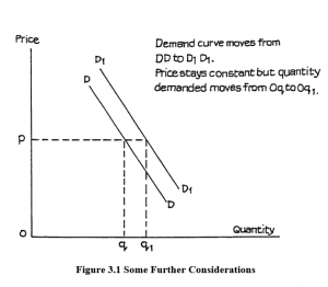
Because a normal two-dimensional graph can cope with only one influence in addition to quantity changes, and because the normal demand curve relates quantity to the product’s own price, a change in quantity demanded brought about by a change in one or more of the other influences has to be represented graphically by a shift in the whole demand curve.

Suppose there is an increase in disposable income which increases the quantity demanded at each price within a given range. This effect can be shown as in Figure 3.1, where the price remains constant at 0p but the increase in income has shifted the curve from DD to D₁D₁, so that the quantity demanded at 0p rises from 0q to 0q₁. A fall in income or a decline in taste, etc. would produce the reverse result, i.e. a shift from D₁D₁to DD.

Remember always to distinguish a movement along a demand curve produced by a change in price (all other influences remaining unchanged) as shown in Figure 2.14 from a shift in the whole curve, showing that demand has moved at all prices within the range under consideration.

It has been argued that the “normal” influences identified above do not tell the full story, and that a fuller understanding of social psychology can give further insights into consumer behaviour. For example, supermarket chains well know the importance of impulse buying, when goods are skilfully displayed. There is also a recognised “snob” effect, when goods may be bought because they are expensive and they appear to be indicators of the owner’s wealth and status. While these considerations are interesting and are clearly of importance to marketing specialists, we can include them under the more general headings of advertising and taste, for the purposes of general analysis of consumer demand.

REVENUE AND REVENUE CHANGES

Total Revenue

Revenue, in general, refers to the money received from the sales of a product. For this reason, the term “sales revenue” is often used. To have any practical meaning, revenue should also be related either to a time period or to a definite quantity of goods sold. For example, a shopkeeper may refer to his weekly sales revenue (the total amounts of sales achieved in a week) or to his revenue from the sales of, say, n pairs of shoes or k kilos of potatoes. A statement that his revenue is RWFy means nothing, unless we can relate it to some quantity of time.

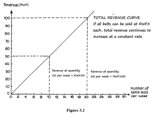
Revenue will not always increase as more goods are sold – this will be the case only if the firm can continue to charge the same price, regardless of quantity it sells. If, say, I make leather belts and can sell all the belts I can make at a standard price of RWF5, then my total revenue is always RWF5 multiplied by whatever quantity I sell.

This can be shown in the form of a total revenue curve, as in Figure 3.2.

However, if I continue to produce more and more belts, there will come a time when customer resistance sets in. I shall have difficulty in finding more people who value belts at this price of RWF5, i.e. the marginal utility of which is at least RWF5. When this time comes, I may still, however, find more people who are willing to pay RWF4.

Now, in the modern world, shopping conditions are often such that I cannot leave my belts un-priced and hope to sort out from the people who visit my shop those willing to pay RWF5 and those willing to pay RWF4. If I want to sell more belts and am willing to charge RWF4, then I must charge this price to everyone. If I continue to produce even more, I might then find that, to sell the increased quantity, I have to charge RWF3. If I go on doing this, I am likely to find that my total revenue starts to fall.

Influences on Price Elasticity of Demand

We have seen that the price elasticity of demand can be expected to change as price changes, so that the product’s own price can normally be regarded as an influence on its elasticity. The important point, really, is whether buyers are likely to pay much attention to the price when deciding whether to buy, or if other influences are more important. These may include current fashion or social attitudes, strong habits (even addiction, in some cases such as tobacco smoking) or the need to buy in order to achieve some other desired objective, such as buying petrol in order to drive to work.

If the product price is only a relatively small amount compared with normal income then price is likely to be less important than the other influences affecting demand, which is thus likely to be price inelastic. Toothbrushes, matches, shoe polish, are all examples of products likely to be price inelastic. Here, high relative price changes at normal price levels are unlikely to weigh heavily with consumers, because annual spending on these items is only a very small part of total income. Other influences, e.g. social attitudes (toothbrushes), smoking decline, the move away from coal fires (matches), and development of non-leather shoes (polish), are likely to be much more important.

We must also be careful to distinguish between the demand elasticity for the class or product and that for a particular brand of the product. My decision whether or not to buy household soap is not likely to be greatly influenced by a 10% rise in its price, but when I am actually making my purchase I am quite likely to compare the prices of two brands and choose the cheaper, assuming that I do not think that one is superior in quality to the other. Thus, demand for a product can be price inelastic, whereas demand for a specific brand of the product can be price elastic. This difference can often be seen in foods. Families may keep to the eating of chicken or beef for dinner and pay roughly the same price for this each week – thus showing a demand price elasticity of around unity. However, the choice of which to buy can be very much influenced by its price, so that we can expect the demand price elasticity for beef and chicken, and certainly for some particular cuts of beef, to be higher than unity, especially if the general level of all meat prices has been rising.

FURTHER DEMAND ELASTICITIES

The general concept of elasticity can be applied to any of the influences on demand. If you think about the concept, you will realise that it is simply the ratio of a proportional change in quantity demanded to the proportional change in the influence considered to be responsible for that quantity movement. The only limiting element in using elasticity is that the influence must be capable of some sort of precise measurement or evaluation. This makes it difficult to produce a definite calculation for, say, changes in taste or fashion, as this is very difficult to measure. The most commonly used elasticities, in addition to the product’s own price, are those for income and for other prices.

Income Elasticity of Demand

This relates to proportional change in quantity demanded to the proportional change in disposable income of customers for the product.

It can be denoted by E_y, so that E_y = proportional change in quantity demanded ÷ proportional change in disposable income.

This may be positive or negative, because there may be an increase in demand following an income increase or a fall in demand. If the income and quantity changes are in the same direction, then the figure for E_y is positive. If the changes are in the opposite directions to each other, then the figure carries the negative sign (₋). A rise in income usually leads to a rise in demand, but demand for some goods may fall. The demand for motor cycles fall as incomes rise and people buy cars. As we saw earlier, such goods are known as inferior goods.

Notice that we are referring here to “disposable income”, i.e. the income left to the consumer after compulsory deductions have been taken. The most important of these are income tax and Social Security contributions. We may also include contributions to pension schemes or to trade unions or professional bodies, where membership is necessary for employment.

In recent years, some economists have argued that we should really be thinking in terms of “discretionary income”. This is the income that is left after all the regular and largely essential household payments have been made, over which the individual has very little control once a particular pattern of life has been chosen. The further deductions which would, then, be made to arrive at discretionary income would be such items as rent or mortgage interest, essential fuel charges (gas and/or electricity) and possibly the cost of travelling to and from work. When these items have all been allowed for, the amount of discretionary income, i.e. the income which people are genuinely free to spend as they choose, is usually very small in relation to the original gross income.

Influences on Income Elasticity of Demand

The following influences are likely to increase a product’s income elasticity of demand:

A high price in relation to income. If a period of saving is required before purchase is possible, or if consumers have to borrow money to obtain a product, then demand can increase only when an income rise makes this possible.
If goods are preferred to “inferior” substitutes, then people may be ready to buy more of these when income increases make this possible.
Association with a higher living standard than that currently enjoyed is likely to lead to rising demand when incomes do rise.

In general, the more highly-priced durable goods (household machines, motor vehicles, etc.) and services are more likely to be income elastic than the staple items of food and clothing. We do not usually buy twice as much of these if we receive double our former income. On the other hand, our spending on holidays may increase by far more than double. Increased spending on motor transport is also associated with rising incomes. Although we have been considering income rises, very similar comments apply to income reductions. Holidays and motor cars are often the first things to be sacrificed in the face of a sudden drop in income.

Cross Elasticity of Demand

This relates the proportional change in demand of one product to the proportional change in price of another.

E_x = proportional change in quantity demanded of X ÷ proportional change in price of Y. Again, the demand movement may be in the same or the opposite direction to the price movement, and the same rules for negative signs apply.

If two products are substitutes for each other, we can expect a rise in price of one to lead to a rise in demand for the other. Beef and pork are in this position, or meat and fish.

If, however, the two products are linked together, e.g. petrol and motor-car tyres, then a rise in price in one leads to a fall in demand for the other, and E_x carries the negative sign (−).

Influences on Cross Elasticity of Demand

The more close substitutes a product has, the more likely it is to react to changes in price of any of those substitutes. The demand for travel by bus reacts to changes in train fares.. Brands of goods are normally much more cross elastic with each other than the good itself is with other goods. We are not unduly influenced by other price movements when we decide how much soap to buy, but we are much more ready to switch to a competing brand when there is a rise in the price of the brand we normally buy.

In the same way, the intensity of negative cross elasticity depends on how closely products are associated with each other.

The Importance of Elasticity Calculations

The calculation of elasticities is not just of academic interest. Anyone, including the business manager and the member of government who wishes to predict accurately the effect of changes in price or income on revenue and on quantities bought, needs to have a clear idea of elasticity and its calculation. If a business manager thinks that a price rise will always increase sales revenue, then he or she needs to be reminded that this is far from being true. A price rise when demand is price elastic will, as you have seen, reduce total sales revenue.

Governments making changes in income or expenditure taxes must be able to calculate their effects on demand. If they do not, then their predictions about the results of the tax change are likely to prove badly out of line with reality.

A government wishing to increase its tax revenue will tend to choose goods the demand for which is price inelastic – tobacco for example, or petrol. If, however, it goes on increasing the tax, the time will eventually come when demand becomes price elastic and any further increase will result in a reduction in sales revenue and a fall in tax receipts. This can be seen by referring to Figure 3.9 where a price rise from, say 5 to 7 will move the good to that part of the demand curve where price rises produce a reduction in total revenue. Price elasticity of demand can also change as a result of other influences. If, for example, there is a long-term trend away from smoking, we can expect demand for cigarettes to become price elastic at lower price levels in the future.

If governments wish to influence consumer demand by price changes, they are likely to try to make demand more price elastic by ensuring that suitable substitutes are available for the target product. For instance, if they wish to reduce consumption of leaded petrol, they must encourage the availability and demand for unleaded petrol, and ensure that vehicle engines can be converted easily and cheaply to unleaded petrol. They may wish to support any tax changes by changes in the law, perhaps requiring all new vehicles to be adapted to use unleaded fuel.

Inelastic Demand and Total Revenue

When demand is Inelastic a Price Increase Raises total Revenue.

Elastic Demand and Total Revenue

When demand is Elastic, a reduction in price increases total revenue.

Unit Demand Elasticity and Total Revenue

When demand is unit elastic, a price change causes no change in total revenue because any price change is cancelled out by an equal and opposite change in Quantity Demanded.

Factors Influencing Demand Elasticity

Availability of Substitutes
The easier it is to switch away from a good the more elastic will its demand be. 2. Time
It is easier to substitute away from a good in the longer-term so demand is more elastic in the long-term
Competitors Policy
If, when one firm changes its price, other firms selling similar goods also change price, demand will be less elastic (i.e. there will be a smaller change in Quantity Demanded.
Percentage of Income Spent on the Good

The higher the percentage spent on the good the more elastic will its demand be.

Income Elasticity of Demand (YED)

Income Elasticity of Demand measures the responsiveness of demand to changes in income.

YED

% Change in Quantity Demanded % Change in Income

Income Elasticity of Demand is normally positive because when incomes rise people consume more of most goods EXCEPT INFERIOR GOODS (e.g. white bread)

If Income Elasticity of Demand is greater than one = income Elastic, i.e. a small change in income causes a bigger change in Quantity Demanded e.g. Luxury Goods and Services.

If Income Elasticity of Demand is less than one = income Inelastic, i.e. a change in income causes a smaller change in Quantity demanded e.g. Basic necessities.

Note: There are always some necessities demanded even at zero income, Luxuries are not demanded until a certain threshold of income has been reached then their demand accelerates as income increases from there.

Cross Price Elasticity of Demand (CED)

Cross Price Elasticity of Demand measures the responsiveness of demand for one good to changes in the price of another good (i.e. a substitute or a complement).

CED

% Change in Quantity Demanded of Good A % Change in Price of Good B

For Substitutes, Cross Price Elasticity of Demand is positive. (e.g. if the price of butter rises

people switch away from butter to margarine so demand for margarine increases

For Complements, Cross Price Elasticity of Demand is negative. (e.g. if price of cars rises, people demand less cars and also less tyres etc.) Elasticity of Supply ( Y^s )

Elasticity of Supply measures the responsiveness of SUPPLY to a change in the price of the good.

Y^s