
THE NEED FOR MEASURES OF LOCATION
We looked at frequency distributions in detail in the previous study unit and you should, by means of a quick revision, make sure that you have understood them before proceeding.
A frequency distribution may be used to give us concise information about its variate, but more often, we will wish to compare two or more distributions. Consider, for example, the distribution of the weights of eggs from two different breeds of poultry (which is a topic in which you would be interested if you were the statistician in an egg marketing company). Having weighed a large number of eggs from each breed, we would have compiled frequency distributions and graphed the results. The two frequency polygons might well look something like Figure 5.1.
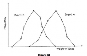
Examining these distributions you will see that they look alike except for one thing – they are located on different parts of the scale. In this case the distributions overlap and, although some eggs from Breed A are of less weight than some eggs from Breed B, eggs from Breed A are, in general, heavier than those from Breed B.
Remember that one of the objects of statistical analysis is to condense unwieldy data so as to make it more readily understood. The drawing of frequency curves has enabled us to make an important general statement concerning the relative egg weights of the two breeds of poultry, but we would now like to take the matter further and calculate some figure which will serve to indicate the general level of the variable under discussion. In everyday life we commonly use such a figure when we talk about the “average” value of something or other. We might have said, in reference to the two kinds of egg, that those from Breed A had a higher average weight than those from Breed B. Distributions with different averages indicate that there is a different general level of the variate in the two groups. The single value which we use to describe the general level of the variate is called a “measure of location” or a “measure of central tendency” or, more commonly, an average.
There are three such measures with which you need to be familiar:
− The arithmetic mean
− The mode − The median.
THE ARITHMETIC MEAN
Introduction
This is what we normally think of as the “average” of a set of values. It is obtained by adding together all the values and then dividing the total by the number of values involved. Take, for example, the following set of values which are the heights, in inches, of seven men:
The Mean of a Grouped Frequency Distribution
Suppose now that you have a grouped frequency distribution. In this case, you will remember, we do not know the actual individual values, only the groups in which they lie. How, then, can we calculate the arithmetic mean? The answer is that we cannot calculate the exact value of x , but we can make an approximation sufficiently accurate for most statistical purposes. We do this by assuming that all the values in any group are equal to the mid-point of that group.
Simplified Calculation
It is possible to simplify the arithmetic still further by the following two devices:
- Work from an assumed mean in the middle of one convenient class.
Work in class intervals instead of in the original units.
Characteristics of the Arithmetic Mean
There are a number of characteristics of the arithmetic mean which you must know and understand. Apart from helping you to understand the topic more thoroughly, the following are the points which an examiner expects to see when he or she asks for “brief notes” on the arithmetic mean:
- It is not necessary to know the value of every item in order to calculate the arithmetic mean. Only the total and the number of items are needed. For example, if you know the total wages bill and the number of employees, you can calculate the arithmetic mean wage without knowing the wages of each person.
- It is fully representative because it is based on all, and not only some, of the items in the distribution.
- One or two extreme values can make the arithmetic mean somewhat unreal by their influence on it. For example, if a millionaire came to live in a country village, the inclusion of his income in the arithmetic mean for the village would make the place seem very much better off than it really was!
- The arithmetic mean is reasonably easy to calculate and to understand.
- In more advanced statistical work it has the advantage of being amenable to algebraic manipulation.
THE MODE
Mode of a Simple Frequency Distribution
The first alternative to the mean which we will discuss is the mode. This is the name given to the most frequently occurring value. Look at the following frequency distribution:
In this case the most frequently occurring value is 1 (it occurred 39 times) and so the mode of this distribution is 1. Note that the mode, like the mean, is a value of the variate, x, not the frequency of that value. A common error is to say that the mode of the above distribution is 39. THIS IS WRONG. The mode is 1. Watch out, and do not fall into this trap!
For comparison, calculate the arithmetic mean of the distribution: it works out at 1.52. The mode is used in those cases where it is essential for the measure of location to be an actually occurring value. An example is the case of a survey carried out by a clothing store to determine what size of garment to stock in the greatest quantity. Now, the average size of garment in demand might turn out to be, let us say, 9.3724, which is not an actually occurring value and doesn’t help us to answer our problem. However, the mode of the distribution obtained from the survey would be an actual value (perhaps size 8) and it would provide the answer to the problem.
Mode of a Grouped Frequency Distribution
When the data is given in the form of a grouped frequency distribution, it is not quite so easy to determine the mode. What, you might ask, is the mode of the following distribution?
A number of procedures based on the frequencies in the groups adjacent to the modal group can be used, and I will now describe one procedure. You should note, however, that these procedures are only mathematical devices for finding the MOST LIKELY position of the mode; it is not possible to calculate an exact and true value in a grouped distribution.
We saw that the modal group of our original distribution was “70-80”. Now examine the groups on each side of the modal group; the group below (i.e. 60-70) has a frequency of 38, and the one above (i.e. 80-90) has a frequency of 20. This suggests to us that the mode may be some way towards the lower end of the modal group rather than at the centre. A graphical method for estimating the mode is shown in Figure 5.2.
This method can be used when the distribution has equal class intervals. Draw that part of the histogram which covers the modal class and the adjacent classes on either side.
Draw in the diagonals AB and CD as shown in Figure 5.2. From the point of intersection draw a vertical line downwards. Where this line crosses the horizontal axis is the mode. In our example the mode is just less than 71.
Characteristics of the Mode
Some of the characteristics of the mode are worth noting as you may well be asked to compare them with those of the arithmetic mean.
- The mode is very easy to find with ungrouped distributions, since no calculation is required.
- It can only be determined roughly with grouped distributions.
- It is not affected by the occurrence of extreme values.
- Unlike the arithmetic mean, it is not based on all the items in the distribution, but only on those near its value.
- In ungrouped distributions the mode is an actually occurring value.
- It is not amenable to the algebraic manipulation needed in advanced statistical work.
- It is not unique, i.e. there can be more than one mode. For example, in the set of numbers, 6, 7, 7, 7, 8, 8, 9, 10, 10, 10, 12, 13, there are two modes, namely 7 and 10. This set of numbers would be referred to as having a bimodal
- The mode may not exist. For example, in the set of numbers 7, 8, 10, 11, 12, each number occurs only once so this distribution has no mode.
THE MEDIAN
Introduction
The desirable feature of any measure of location is that it should be near the middle of the distribution to which it refers. Now, if a value is near the middle of the distribution, then we expect about half of the distribution to have larger values, and the other half to have smaller values. This suggests to us that a possible measure of location might be that value which is such that exactly half (i.e. 50%) of the distribution has larger values and exactly half has lower values. The value which so divides the distribution into equal parts is called the MEDIAN. Look at the following set of values:
6, 7, 7, 8, 8, 9, 10, 10, 10, 12, 13
The total of these eleven numbers is 100 and the arithmetic mean is therefore 100/11 = 9.091, while the mode is 10 because that is the number which occurs most often (three times). The median, however, is 9 because there are five values above and five values below 9. Our first rule for determining the median is therefore as follows:
Arrange all the values in order of magnitude and the median is then the middle value.
Note that all the values are to be used: even though some of them may be repeated, they must all be put separately into the list. In the example just dealt with, it was easy to pick out the middle value because there was an odd number of values. But what if there is an even number? Then, by convention, the median is taken to be the arithmetic mean of the two values in the middle. For example, take the following set of values: 6, 7, 7, 8, 8, 9, 10, 10, 11, 12
The two values in the middle are 8 and 9, so that the median is 8.5
Median of a Simple Frequency Distribution
Statistical data, of course, is rarely in such small groups and, as you have already learned, we usually deal with frequency distributions. How, then do we find the median if our data is in the form of a distribution?
Let us take the example of the frequency distribution of accidents already used in discussing the mode. The total number of values is 123 and so when those values are arranged in order of magnitude, the median will be the 62nd item because that will be the middle item. To see what the value of the 62nd item will be, let us again draw up the distribution:
Median of a Grouped Frequency Distribution
The final problem connected with the median is how to find it when our data is in the form of a grouped distribution. The solution to the problem, as you might expect, is very similar to the solution for an ungrouped distribution; we halve the total frequency and then find, from the cumulative frequency column, the corresponding value of the variate.
Because a grouped frequency distribution nearly always has a large total frequency, and because we do not know the exact values of the items in each group, it is not necessary to find the two middle items when the total frequency is even: just halve the total frequency and use the answer (whether it is a whole number or not) for the subsequent calculation.
Characteristics of the Median
Characteristic features of the median, which you should compare with those of the mean and the mode, are as follows:
- It is fairly easily obtained in most cases, and is readily understood as being the “halfway point”.
- It is less affected by extreme values than the mean. The millionaire in the country village might alter considerably the mean income of the village but he would have almost no effect at all on the median.
- It can be obtained without actually having all the values. If, for example, we want to know the median height of a group of 21 men, we do not have to measure the height of every single one; it is only necessary to stand the men in order of their heights and then only the middle one (No. 11) need be measured, for his height will be the median height. The median is thus of value when we have open-ended classes at the edges of the distribution as its calculation does not depend on the precise values of the variate in these classes, whereas the value of the arithmetic mean does.
- The median is not very amenable to further algebraic manipulation.