INTRODUCTION TO DISPERSION
In order to get an idea of the general level of values in a frequency distribution, we have studied the various measures of location that are available. However, the figures which go to make up a distribution may all be very close to the central value, or they may be widely dispersed about it, e.g. the mean of 49 and 51 is 50, but the mean of 0 and 100 is also 50! You can see, therefore, that two distributions may have the same mean but the individual values may be spread about the mean in vastly different ways.
When applying statistical methods to practical problems, a knowledge of this spread (which we call “dispersion” or “variation”) is of great importance. Examine the figures in the following table:
Although the two factories have the same mean output, they are very different in their week-to-week consistency. Factory A achieves its mean production with only very little variation from week to week, whereas Factory B achieves the same mean by erratic upsand-downs from week to week. This example shows that a mean (or other measure of location) does not, by itself, tell the whole story and we therefore need to supplement it with a “measure of dispersion”.
As was the case with measures of location, there are several different measures of dispersion in use by statisticians. Each has its own particular merits and demerits, which will be discussed later. The measures in common use are:
− Range
− Quartile deviation
− Mean deviation
− Standard deviation
−
We will discuss three of these here.
THE RANGE
This is the simplest measure of dispersion; it is simply the difference between the largest and the smallest. In the example just given, we can see that the lowest weekly output for Factory A was 90 and the highest was 107; the range is therefore 17. For Factory B the range is 156 – 36 = 120. The larger range for Factory B shows that it performs less consistently than Factory A.
The advantage of the range as a measure of the dispersion of a distribution is that it is very easy to calculate and its meaning is easy to understand. For these reasons it is used a great deal in industrial quality control work. Its disadvantage is that it is based on only two of the individual values and takes no account of all those in between. As a result, one or two extreme results can make it quite unrepresentative. Consequently, the range is not much used except in the case just mentioned.
THE QUARTILE DEVIATION, DECILES AND PERCENTILES
The Quartile Deviation
This measure of dispersion is sometimes called the “semi-interquartile range”. To understand it, you must cast your mind back to the method of obtaining the median from the ogive. The median, you remember, is the value which divides the total frequency into two halves. The values which divide the total frequency into quarters are called quartiles and they can also be found from the ogive
Calculation of the Quartile Deviation
The quartile deviation is not difficult to calculate and some examination questions may specifically ask for it to be calculated, in which case a graphical method is not acceptable. Graphical methods are never quite as accurate as calculations.
Deciles and Percentiles
It is sometimes convenient, particularly when dealing with wages and employment statistics, to consider values similar to the quartiles but which divide the distribution more finely. Such partition values are deciles and percentiles. From their names you will probably have guessed that the deciles are the values which divide the total frequency into tenths and the percentiles are the values which divide the total frequency into hundredths. Obviously it is only meaningful to consider such values when we have a large total frequency.
THE STANDARD DEVIATION
Most important of the measures of dispersion is the standard deviation. Except for the use of the range in statistical quality control and the use of the quartile deviation in wages statistics, the standard deviation is used almost exclusively in statistical practice. It is defined as the square root of the variance and so we need to know how to calculate the variance first.
The Variance
We start by finding the deviations from the mean, and then squaring them, which removes the negative signs in a mathematically acceptable fashion,
Standard Deviation of a Simple Frequency Distribution
If the data had been given as a frequency distribution (as is often the case) then only the different values would appear in the “x” column and we would have to remember to multiply each result by its frequency:
Standard Deviation of a Grouped Frequency Distribution
When we come to the problem of finding the standard deviation of a grouped frequency distribution, we again assume that all the readings in a given group fall at the mid-point of the group, so we can find the arithmetic mean as before
Characteristics of the Standard Deviation
In spite of the apparently complicated method of calculation, the standard deviation is the measure of dispersion used in all but the very simplest of statistical studies. It is based on all of the individual items, it gives slightly more emphasis to the larger deviations but does not ignore the smaller ones and, most important, it can be treated mathematically in more advanced statistics.
THE COEFFICIENT OF VARIATION
Suppose that we are comparing the profits earned by two businesses. One of them may be a fairly large business with average monthly profits of RWF50,000, while the other may be a small firm with average monthly profits of only RWF2,000. Clearly, the general level of profits is very different in the two cases, but what about the month-by-month variability? We will compare the two firms as to their variability by calculating the two standard deviations; let us suppose that they both come to RWF500. Now, RWF500 is a much more significant amount in relation to the small firm than it is in relation to the large firm so that, although they have the same standard deviations, it would be unrealistic to say that the two businesses are equally consistent in their month-to-month earnings of profits. To overcome the difficulty, we express the SD as a percentage of the mean in each case and we call the result the “coefficient of variation”.
Applying the idea to the figures which we have just quoted, we get coefficients of variation (usually indicated in formulae by V or CV) as follows:
This shows that, relatively speaking, the small firm is more erratic in its earnings than the large firm.
Note that although a standard deviation has the same units as the variate, the coefficient of variation is a ratio and thus has no units.
Another application of the coefficient of variation comes when we try to compare distributions the data of which are in different units as, for example, when we try to compare a French business with an American business. To avoid the trouble of converting the dollars to euro (or vice versa) we can calculate the coefficients of variation in each case and thus obtain comparable measures of dispersion.
SKEWNESS
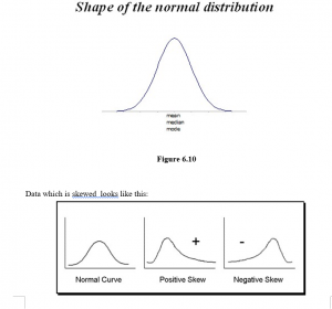
When the items in a distribution are dispersed equally on each side of the mean, we say that the distribution is symmetrical. Figure 6.2 shows two symmetrical distributions.
When the items are not symmetrically dispersed on each side of the mean, we say that the distribution is skew or asymmetric.
A distribution which has a tail drawn out to the right is said to be positively skew, while one with a tail to the left, is negatively skew. Two distributions may have the same mean and the same standard deviation but they may be differently skewed. This will be obvious if you look at one of the skew distributions in Figure 6.3 and then look at the same one through from the other side of the paper!
What, then, does skewness tell us? It tells us that we are to expect a few unusually high values in a positively skew distribution or a few unusually low values in a negatively skew distribution.
If a distribution is symmetrical, the mean, mode and median all occur at the same point, i.e. right in the middle. But in a skew distribution the mean and the median lie somewhere along the side of the “tail”, although the mode is still at the point where the curve is highest. The more skewed the distribution, the greater the distance from the mode to the mean and the median, but these two are always in the same order; working outwards from the mode, the median comes first and then the mean – see Figure 6.4.
For most distributions, except for those with very long tails, the following relationship holds approximately:
Mean – Mode = 3(Mean – Median)
The more skew the distribution, the more spread out are these three measures of location, and so we can use the amount of this spread to measure the amount of skewness. The most usual way of doing this is to calculate
You are expected to use one of these formulae when an examiner asks for the skewness (or “coefficient of skewness”, as some of them call it) of a distribution. When you do the calculation, remember to get the correct sign (+ or –) when subtracting the mode or median from the mean and then you will get negative answers from negatively skew distributions, and positive answers for positively skew distributions. The value of the coefficient of skewness is between –3 and +3, although values below –1 and above +1 are rare and indicate very skewed distributions.
Examples of variates with positive skew distributions include size of incomes of a large group of workers, size of households, length of service in an organisation, and age of a workforce. Negative skew distributions occur less frequently. One such example is the age at death for the adult population in Rwanda.
AVERAGES AND MEASURES OF DISPERSION
Measures of Central Tendency and Dispersion
- Averages and variations for ungrouped and grouped data.
- Special cases such as the Harmonic mean and the geometric mean
In the last section we described data using graphs, histograms and Ogives mainly for grouped numerical data. Sometimes we do not want a graph; we want one figure to describe the data.
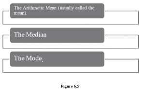
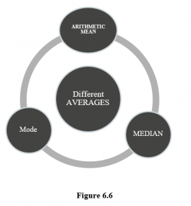
One such figure is called the average. There are three different averages, all summarise the data with just one figure but each one has a different interpretation.
When describing data the most obvious way and the most common way is to get an average figure. If I said the average amount of alcohol consumed by Rwandan women is 2.6 units per week then how useful is this information? Usually averages on their own are not much use; you also need a measure of how spread out the data is. We will deal with the spread of the data later.
What is the best average, if any, to use in each of the following situations? Justify each of your answers.
- To establish a typical wage to be used by an employer in wage negotiations for a small company of 300 employees, a few of whom are very highly paid specialists.
- To determine the height to construct a bridge (not a draw bridge) where the distribution of the heights of all ships which would pass under is known and is skewed to the right.
There are THREE different measures of AVEARGE, and three different measures of dispersion. Once you know the mean and the standard deviation you can tell much more about the data than if you have the average only.
The Median and the Quartiles.
The median is the figure where half the values of the data set lie below this figure & half above. In a class of students the median age would be the age of the person where half the class is younger than this person and half older. It is the age of the middle aged student.
If you had a class of 11 students, to find the median age, you would line up all the students starting with the youngest to the oldest. You would then count up to the middle person, the 5th one along, ask them their age and that is the median age.
To find the median of raw data you need to firstly rank the figures from smallest to highest and then choose the middle figure.
For grouped data it is not as easy to rank the data because you don’t have single figures you have groups. There is a formula which can be used or the median can be found from the ogive. From the ogive, you go to the half way point on the vertical axis (if this is already in percentages then up to 50%) and then read the median off the horizontal axis.
The Mode
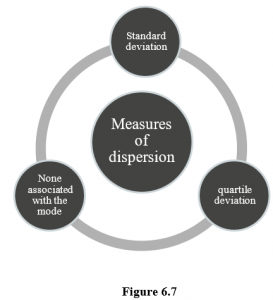
There is no measure of dispersion associated with the mode.
The mode is the most frequently occurring figure in a data set. There is often no mode particularly with continuous data or there could be a few modes. For raw data you find the mode by looking at the data as before, or by doing a tally.
For grouped data you can estimate the mode from a histogram by finding the class with the highest frequency and then estimating.
- Measures of dispersion- range, variance, standard deviation, co-efficient of variation.
The range is explained earlier it is found crudely by taking the highest figure in the data set and subtracting the lowest figure.
The variance is very similar to the standard deviation and measures the spread of the data. If I had two different classes and the mean result in both classes was the same, but the variance was higher in class B then results in class B were more spread out. The variance is found by getting the standard deviation and squaring it.
The standard deviation is done already.
The co-efficient of variation is used to establish which of two sets of data is relatively more variable.
For example, take two companies ABC and CBA. You are given the following information about their share price and the standard deviation of share price over the past year.
The Harmonic mean: The harmonic mean is used in particular circumstances namely when data consists of a set of rates such as prices, speed or productivity.
Dispersion and Skewness:
The normal distribution is used frequently in statistics. It is not skewed and the mean, median and the mode will all have the same value. So for normally distributed data it does not matter which measure of average you use as they are all the same.