Investment appraisal

Introduction – Investment, financing and dividend decisions
Three of the key decisions facing the financial manager (identified in Chapter 1
above) are:
Investment – what projects should be undertaken by the organisation?
Finance – how should the necessary funds be raised?
Dividends – how much cash should be allocated each year to be paid as a
return to shareholders, and how much should be retained to meet the cash
needs of the business?
This chapter and the next three chapters of this Text cover these three key
decisions in detail.
However, as well as considering these three areas separately, it is vital that we
understand that the three decisions are very closely interlinked.
Examples of links between these three key decisions
Investment decisions cannot be taken without consideration of where and how
the funds are to be raised to finance them. The type of finance available will, in
turn, depend to some extent on the nature of the project – its size, duration, risk,
capital asset backing, etc.
Dividends represent the payment of returns on the investment back to the
shareholders, the level and risk of which will depend upon the project itself, and
how it was financed.
Debt finance, for example, can be cheap (particularly where interest is tax
deductible) but requires an interest payment to be made out of project earnings,
which can increase the risk of the shareholders’ dividends.
Throughout this chapter and the next three, it is critical that we continue to
consider these inter-relationships. Exam questions rarely focus on just a single
area of the syllabus, so we must consider such links throughout in order to
prepare fully for the exam.

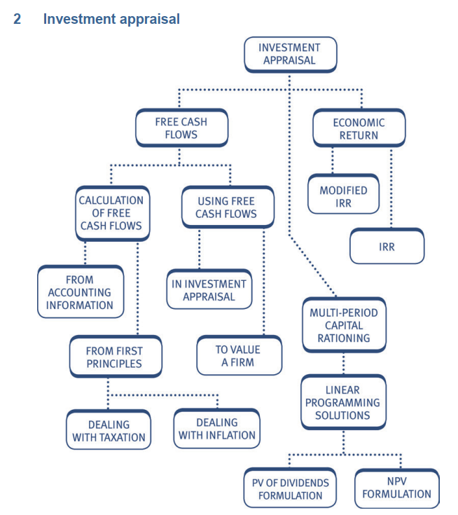
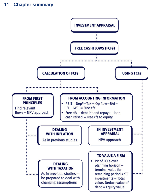
A key concept in investment appraisal – Free cash flow
Cash that is not retained and reinvested in the business is called free cash
flow.
It represents cash flow available:
• to all the providers of capital of a company
• to pay dividends or finance additional capital projects.

Uses of free cash flows
Free cash flows are used frequently in financial management:
• as a basis for evaluating potential investment projects – see below
• as an indicator of company performance – see Chapter 14: Corporate
failure and reconstruction
• to calculate the value of a firm and thus a potential share price – see
Chapter 13: Business valuation.
Calculating free cash flows for investment appraisal
Free cash flows can be calculated simply as:
Free cash flow = Revenue – Costs – Investments
The free cash flows used to evaluate investment projects are therefore
essentially the net relevant cash flows you will recall from your earlier studies.
Use of free cash flows in investment appraisal
This chapter covers the following investment appraisal methods, all of which
incorporate the use of free cash flows:
• Net Present Value (NPV)
• Internal Rate Of Return (IRR)
• Modified Internal Rate Of Return (MIRR)
• Discounted Payback Period
• Duration (Macaulay Duration and Modified Duration).
4 Net Present Value
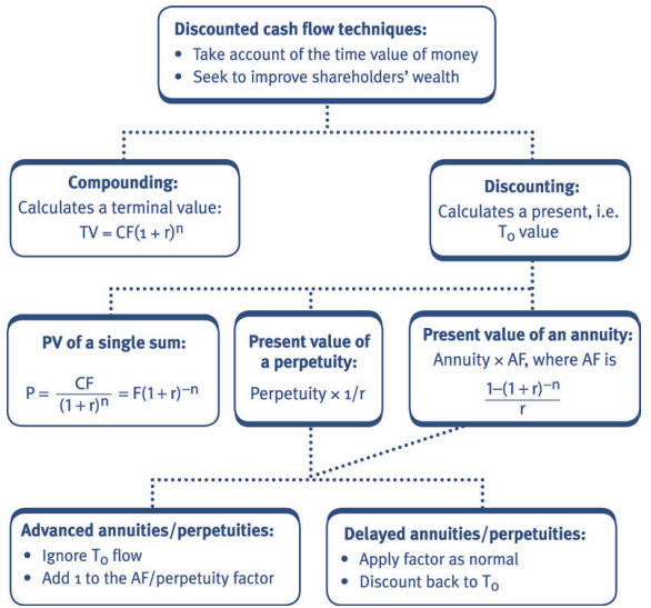
Capital investment projects are best evaluated using the net present value
(NPV) technique. You should recall from earlier studies that this involved
discounting the relevant cash flows for each year of the project at an
appropriate cost of capital.
As mentioned above the net relevant cash flows associated with the project are
the free cash flows it generates. The discounted free cash flows are totalled to
provide the NPV of the project.
Some basic NPV concepts (relevant cash flows, discounting, the impact of
inflation, the impact of taxation) are covered below.

Relevant cash flows

Relevant costs and revenues Relevant cash flows are those costs and revenues that are: • future • incremental. Some basic NPV concepts are revised as follows: You should therefore ignore: • sunk costs • committed costs • non-cash items • apportioned overheads.

 

Discounting

The impact of inflation

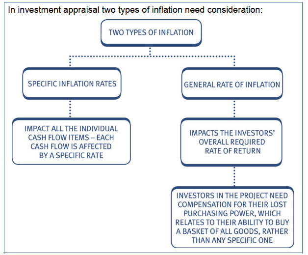
The treatment of inflation was introduced in the Financial Management syllabus. A brief recap follows: Inflation is a general increase in prices leading to a general decline in the real value of money. In times of inflation, the fund providers will require a return made up of two elements: • Real return for the use of their funds. • Additional return to compensate for inflation. The overall required return is called the money or nominal rate of return. Real and nominal rates are linked by the Fisher formula: (1 + i) = (1 + r)(1 + h) Or (1 + r) = (1 + i)/(1 + h) in which: r = real rate i = money/nominal interest rate h = general inflation rate.

Calculating the free cash flows of a project under inflation
In project appraisal the impact of inflation must be taken into account when
calculating the free cash flows to be discounted.
The impact of inflation can be dealt with in two different ways – both methods
give the same NPV.

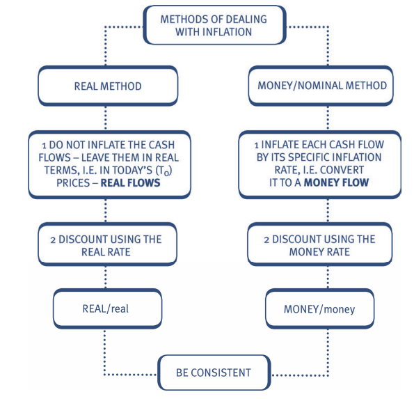
Note:
• The real method can only be used if all cash flows are inflating at the
general rate of inflation.
• In questions involving specific inflation rates, taxation or working
capital, the money/nominal method is usually more reliable.

Illustration of inflation in investment appraisal

A company is considering investing $4.5m in a project to achieve an annual increase in revenues over the next five years of $2m. The project will lead to an increase in wage costs of $0.4m pa and will also require expenditure of $0.3m pa to maintain the level of existing assets to be used on the project. Additional investment in working capital equivalent to 10% of the increase in revenue will need to be in place at the start of each year.

The following forecasts are made of the rates of inflation each year for the
next five years:

Revenues Wages Assets General prices

10% 5% 7% 6.5%

The real cost of capital of the company is 8%.
All cash flows are in real terms. Ignore tax.
Find the free cash flows of the project and determine whether it is
worthwhile.
Solution
$000

T0	T1	T2	T3	T4	T5
Increased revenues (infl. @ 10%) Increased wage costs (infl. @ 5%)
2,200	2,420	2,662	2,928	3,221
(420) ––––– 1,780	(441) ––––– 1,979	(463) ––––– 2,199	(486) ––––– 2,442	510) ––––– 2,711
–––––
Operating cash flows New investment Asset replacement spending (infl. @ 7%) Working capital injection (W1)
(4,500)
(321)	(343)	(367)	(393)	(421)
(220) ––––– (4,720)	(22) ––––– 1,437	(24) ––––– 1,612	(27) ––––– 1,805	(29) ––––– 2,020	322 ––––– 2,612
Free cash flows PV factor @ 15% (W2)
1.000 ––––– (4,720) –––––	0.870 ––––– 1,250 –––––	0.756 ––––– 1,219 –––––	0.658 ––––– 1,187 –––––	0.572 ––––– 1,155 –––––	0.497 ––––– 1,298 –––––
PV of free cash flows

The NPV = $1,389,000 which suggests that the project is worthwhile.
(W1) Working capital injection

T0	T1	T2	T3	T4	T5
Increased revenues Working capital required 10% in advance Working capital injection (W2) Cost of capital	2,200	2,420	2,662	2,928	3,221
220	242	266	293	322
(220)	(22)	(24)	(27)	(29)	322

(1 + i) = (1 + r) (1 + h) = (1.08) (1.065) = 1.15, giving i = 15%

Test your understanding 1 – NPV with inflation revision

A company plans to invest $7m in a new product. Net contribution over the next five years is expected to be $4.2m pa in real terms. Marketing expenditure of $1.4m pa will also be needed. Expenditure of $1.3m pa will be required to replace existing assets which will now be used on the project but are getting to the end of their useful lives. This expenditure will be incurred at the start of each year. Additional investment in working capital equivalent to 10% of contribution will need to be in place at the start of each year. Working capital will be released at the end of the project. The following forecasts are made of the rates of inflation each year for the next five years: The real cost of capital of the company is 6%. All cash flows are in real terms. Ignore tax. Required: Forecast the free cash flows of the project and determine whether it is worthwhile using the NPV method.

Contribution 8%
Marketing 3%
Assets 4%
General prices 4.7%
The impact of taxation
There are two main impacts of taxation in an investment appraisal:
• tax is charged on operating cash flows, and
• tax allowable depreciation (sometimes referred to as capital allowances or
writing down allowances) can be claimed, thus generating tax relief.

Revision of taxation on operating cash flows

Tax on operating flows Corporation tax charged on a company’s profits is a relevant cash flow for NPV purposes. It is assumed that: • operating cash inflows will be taxed at the corporation tax rate • operating cash outflows will be tax deductible and attract tax relief at the corporation tax rate • tax is paid in the same year the related operating cash flow is earned unless otherwise stated • investment spending attracts tax allowable depreciation which gets tax relief (see the section below) • the company is earning net taxable profits overall.

 

Revision of Tax Allowable Depreciation

For tax purposes, a business may not deduct the cost of an asset from its profits as depreciation (in the way it does for financial accounting purposes). Instead the cost must be deducted in the form of tax allowable depreciation (TAD). The basic rules that follow are based on the current UK tax legislation: • TAD is calculated on a reducing balance basis. • The total TAD given over the life of an asset equates to the fall in value over the period (i.e. the cost less any scrap proceeds). • TAD is claimed as early as possible. • TAD is given for every year of ownership except the year of disposal.

• In the year of sale or scrap a balancing allowance or charge arises.
$
Original cost of asset X
Cumulative TAD claimed (X)
–––
Written down value of the asset X
Disposal value of the asset (X)
–––
Balancing allowance or charge X
–––

You should carefully check the information given in the question however,
since the examiner could ask you to examine the impact on the project of
potential changes in the rules, for example:
• giving 50% TAD in the first year of ownership and 25% thereafter
• giving 100% first year TAD allowances (these are sometimes
available to encourage investment in certain areas or types of
assets)
• changing the calculation method from reducing balance to straight
line.
Calculating the free cash flows of a project taking account of taxation
In project appraisal the effects of taxation must be taken into account when
calculating the free cash flows to be discounted.

Illustration of taxation in investment appraisal

A company buys an asset for $26,000. It will be used on a project for three years after which it will be disposed of on the final day of year 3 for $12,500. Tax is payable at 30%. Tax allowable depreciation is available at 25% reducing balance, and a balancing allowance or charge should be calculated when the asset is sold. Net trading income from the project is $16,000 p.a. and the cost of capital is 8%. Required: Forecast the free cash flows of the project and determine whether it is worthwhile using the NPV method. Solution

Time $
T0 Initial investment 26,000
T1 TAD @ 25% (6,500)
––––––
Written down value 19,500
T2 TAD @ 25% (4,875)
––––––
Written down value 14,625
Sale proceeds (12,500)
––––––
T3 Balancing allowance 2,125

NPV calculation

Time	T0	T1	T2	T3
Net trading inflows TAD (from working)	16,000 6,500 –––––– 9,500 (2,850) 6,500	16,000 4,875 –––––– 11,125 (3,338) 4,875	16,000 2,125 –––––– 13,875 (4,163) 2,125
––––––
Taxable profit Tax payable (30%) Add back TAD Initial investment Scrap proceeds
(26,000)
12,500 –––––– 24,337
–––––– (26,000)	–––––– 13,150	–––––– 12,662
Free cash flows Discount factor @ 8%
1.000 –––––– (26,000) –––––– 16,353 ––––––	0.926 –––––– 12,177 ––––––	0.857 –––––– 10,852 ––––––	0.794 –––––– 19,324 ––––––
Present value
NPV

 

Test your understanding 2 – NPV with taxation revision

A project will require an investment in a new asset of $10,000. It will be used on a project for four years after which it will be disposed of on the final day of year 4 for $2,500. Tax is payable at 30% one year in arrears. Tax allowable depreciation is available at 25% (reducing balance), and a balancing allowance or charge should be calculated when the asset is sold. Net operating flows from the project are expected to be $4,000 pa. The company’s cost of capital is 10%. Ignore inflation. Required: Forecast the free cash flows of the project and determine whether it is worthwhile using the NPV method.

nterpreting the IRR
The IRR provides a decision rule for investment appraisal, but also provides
information about the riskiness of a project – i.e. the sensitivity of its returns.
The project will only continue to have a positive NPV whilst the firm’s cost of
capital is lower than the IRR.
A project with a positive NPV at 14% but an IRR of 15% for example, is clearly
sensitive to:
• an increase in the cost of finance
• an increase in investors’ perception of the potential risks
• any alteration to the estimates used in the NPV appraisal.

Interpretation of IRR

Increases in interest rates will clearly increase the company’s costs of finance as will concerns affecting the stock market as a whole and hence the returns demanded by investors. However, other, company specific factors – such as the actions of competitors may affect the firm’s position in the market place and the viability of its business model. This could impact the level of systematic risk it faces and result in an increase in the required return of shareholders. Where the IRR is close to the company cost of capital, any changes to estimates in the NPV calculation will have a significant impact on the viability of the project. Any unexpected changes such as an increase in the costs of raw materials, or an aggressive advertising campaign run by a competitor will erode the return margin and may make the project unacceptable to investors.

6 The modified IRR (MIRR)
Problems with using IRR
There are a number of problems with the standard IRR calculation:
• The assumptions. IRR is often mistakenly assumed to be a measure of the
return from a project, which it is not. The IRR only represents the return
from the project if funds can be reinvested at the IRR for the duration of
the project.

The decision rule is not always clear cut. For example, if a project has
2 IRRs (or more), it is difficult to interpret the rule which says “accept the
project if the IRR is higher than the cost of capital”.
• Choosing between projects. Since projects can have multiple IRRs (or
none at all) it is difficult to usefully compare projects using IRR.
It is therefore usually considered more reliable to calculate the NPV of projects
for investment appraisal purposes.

More on the problems with IRR

For conventional projects (those with a cash outflow at time 0 followed by inflows over the life of the project), the decision rule states that projects should be accepted if the IRR exceeds the cost of capital. However unconventional projects with different cash flow patterns may have no IRR, more than one IRR, or a single IRR but the project should only be accepted if the cost of capital is greater. The IRR calculates the discount rate that would cause the project to break-even assuming it: • is the cost of financing the project • is the return that can be earned on all the returns earned by the project. Since, in practice, these rates are likely to be different, the IRR is unreliable. A project with a high IRR is not necessarily the one offering the highest return in NPV terms and IRR is therefore an unreliable tool for choosing between mutually exclusive projects.

A more useful measure is the modified internal rate of return or MIRR.
This measure has been developed to counter the above problems since it:
• is unique
• gives a measure of the return from a project
• is a simple percentage.
It is therefore more popular with non-financially minded managers, as a simple
rule can be applied:
MIRR = Project’s return
If Project return > company cost of finance  Accept project

The interpretation of MIRR
MIRR measures the economic yield of the investment under the assumption
that any cash surpluses are reinvested at the firm’s current cost of capital.
Although MIRR, like IRR, cannot replace net present value as the principle
evaluation technique it does give a measure of the maximum cost of finance
that the firm could sustain and allow the project to remain worthwhile. For this
reason it gives a useful insight into the margin of error, or room for negotiation,
when considering the financing of particular investment projects.
Calculation of MIRR
There are several ways of calculating the MIRR, but the simplest is to use the
following formula which is provided on the formula sheet in the exam:
MIRR = [PVR/PVI]1/n(1 + re) –1
where
PVR = the present value of the ‘return phase’ of the project
PVI = the present value of the ‘investment phase’ of the project
re = the firm’s cost of capital.
Student Accountant article
Read the article ‘Modified internal rate of return’ in the Technical Articles section
of the ACCA website for more details on MIRR.

Test your understanding 4

A project with the following cash flows is under consideration: Cost of capital 8% Required: Calculate the MIRR.

$000 T0 T1 T2 T3 T4
(20,000) 8,000 12,000 4,000 2,000
Discounted Payback Period (DPP)
Traditional payback period
The payback period was introduced in Financial Management (FM).
Payback period measures the length of time it takes for the cash returns from a
project to cover the initial investment.
The main problem with payback period is that it does not take account of the
time value of money.
Discounted payback period
Hence, the discounted payback period can be computed instead.
Discounted payback period measures the length of time before the discounted
cash returns from a project cover the initial investment.
The shorter the discounted payback period, the more attractive the project is.
A long discounted payback period indicates that the project is a high risk
project.

Illustration 1 – Discounted Payback Period

A project with the following cash flows is under consideration: Cost of capital 8% Required: Calculate the Discounted Payback Period. Solution 0 (20,000) (20,000) 1 8,000/(1.08) = 7,407 (12,593) 2 12,000/(1.08)2 = 10,288 (2,305) 3 4,000/(1.08)3 = 3,175 870 Hence discounted payback period = 2 years + (2,305/3,175) = 2.73 years

$000 T0 T1 T2 T3 T4
(20,000) 8,000 12,000 4,000 2,000
Year Discounted cash flow Cumulative discounted
cash flow
Duration (Macaulay duration)
Introduction to the concept of duration
Duration measures the average time to recover the present value of the project
(if cash flows are discounted at the cost of capital).
Duration captures both the time value of money and the whole of the cash flows
of a project. It is also a measure which can be used across projects to indicate
when the bulk of the project value will be captured.
Projects with higher durations carry more risk than projects with lower durations.
Calculation of duration
There are several different ways of calculating duration, the most common of
which is Macaulay duration, illustrated below.

More details on duration

As mentioned above, duration measures the average time to recover the present value of the project if discounted at the cost of capital. However, if cash flows are discounted at the project’s IRR, it can be used to measure the time to recover the initial investment. As well as being used in project appraisal, duration is commonly used to assess the likely volatility (risk) associated with corporate bonds. An example of duration in the context of bonds is shown in Chapter 8.

 

Payback, discounted payback and duration

Payback, discounted payback and duration are three techniques that measure the return to liquidity offered by a capital project. In theory, a firm that has ready access to the capital markets should not be concerned about the time taken to recapture the investment in a project. However, in practice managers prefer projects to appear to be successful as quickly as possible. Payback period Payback as a technique fails to take into account the time value of money and any cash flows beyond the project date. It is used by many firms as a coarse filter of projects and it has been suggested to be a proxy for the redeployment real option.

Discounted payback period
Discounted payback does surmount the first difficulty but not the second
in that it is still possible for projects with highly negative terminal cash
flows to appear attractive because of their initial favourable cash flows.
Conversely, discounted payback may lead a project to be discarded that
has highly favourable cash flows after the payback date.
Duration
Duration measures either the average time to recover the initial
investment (if discounted at the project’s internal rate of return) of a
project, or to recover the present value of the project if discounted at the
cost of capital. Duration captures both the time value of money and the
whole of the cash flows of a project. It is also a measure which can be
used across projects to indicate when the bulk of the project value will be
captured.
Its disadvantage is that it is more difficult to conceptualise than payback
and may not be employed for that reason.

Illustration 2 – Macaulay duration

A project with the following cash flows is under consideration: Cost of capital 8% Required: Calculate the project’s Macaulay duration. Solution The Macaulay duration is calculated by first calculating the discounted cash flow for each future year, and then weighting each discounted cash flow according to its time of receipt, as follows: Next, the sum of the (PV × Year) figures is found, and divided by the present value of these ‘return phase’ cash flows. Sum of (PV × Year) figures = 7,408 + 20,568 + 9,528 + 5,880 = 43,384 Present value of return phase cash flows = 7,408 + 10,284 + 3,176 + 1,470 = 22,338 Hence, the Macaulay duration is 43,384/22,338 = 1.94 years

$000 T0 T1 T2 T3 T4
(20,000) 8,000 12,000 4,000 2,000
$000 T0 T1 T2 T3 T4
Cash flow 8,000 12,000 4,000 2,000
D F @ 8% 0.926 0.857 0.794 0.735
PV @ 8% 7,408 10,284 3,176 1,470
PV × Year 7,408 20,568 9,528 5,880

Test your understanding 5

A project with the following cash flows is under consideration: $m T0 T1 T2 T3 T4 T5 T6 Net cash flow (127) (37) 52 76 69 44 29 Cost of capital 10% Calculate the project’s discounted payback period and Macaulay duration.

 

Modified Duration

As well as the Macaulay Duration, there is another commonly used measure of duration, known as Modified Duration. Comparison of Macaulay Duration and Modified Duration Macaulay Duration is the name given to the weighted average time until cash flows are received, and is measured in years. Modified Duration is the name given to the price sensitivity and is the percentage change in price for a unit change in yield. Macaulay Duration and Modified Duration differ slightly, and there is a simple relationship between the two (assuming that cash flows are discounted annually), namely: Modified Duration = Macaulay Duration/(1+ cost of capital) Therefore, in the above illustration, where the project cash flows were discounted at 8% and the Macaulay Duration was 1.94 years, the Modified Duration is (1.94/1.08 =) 1.80.

9 Investment appraisal and capital rationing
Capital rationing was first introduced in Financial Management (FM). A brief
recap follows:
Capital rationing – The basics
Shareholder wealth is maximised if a company undertakes all possible positive
NPV projects.
Capital rationing is where there are insufficient funds to do so.
This shortage of funds may be for:
• a single period only – dealt with as in limiting factor analysis by calculating
profitability indexes (PIs)
PI = NPV/PV of capital invested
• more than one period – extending over a number of years or even
indefinitely.

Test your understanding 6 – Single period capital rationing

Peel Co has identified 4 positive NPV projects, as follows: (ii) independent and indivisible (iii) mutually exclusive.

Project NPV ($m) Investment at t0 ($m)
A 60 9
B 40 12
C 35 6
D 20 4
Peel Co can only raise $12m of finance to invest at t0.
Required:
Advise the company which project(s) to accept if the projects are:
(i) independent and divisible
Multi-period capital rationing
A solution to a multi-period capital rationing problem cannot be found using PIs.
This method can only deal with one limiting factor (i.e. one period of shortage).
Here there are a number of limiting factors (i.e. a number of periods of
shortage) and linear programming techniques must therefore be applied.
In the exam you will not be expected to produce a solution to a linear
programming problem, but you may be asked to formulate the linear
programme.
In practice, long term capital rationing is a signal that the firm should be looking
to expand its capital base through a new issue of finance to the markets.

Revision of linear programming (LP)

In your previous studies, you were introduced to the details of linear programming. In AFM, we are interested only in formulating the linear programming problem and this revision example therefore only reviews those first key stages. Linear programming is a technique for dealing with scarce or rationed resources. The solution calculated identifies the optimum allocation of the scarce resources between the products/projects being considered. A brief recap follows: The linear programme is formulated in three stages: (1) Define the unknowns. (2) Formulate the objective function. (3) Express the constraints in terms of inequalities including the non negativities.

Simple LP example

A company makes two products, brooms and mops. Each product passes through two departments, manufacture and packaging. The time spent in each department is as follows: Departmental time (hours) Manufacture Packaging Brooms 3 2 Mops 4 6 There are 4,800 hours available in the manufacturing department and 3,600 available in the packaging department. Production of brooms must not exceed 1,100 units. The contribution earned from one broom is $15 and from a mop is $10. Formulate the linear programme needed to identify the optimum use of the scarce labour resource. Solution (1) Define the unknowns Let m = number of mops to be produced. Let b = number of brooms to be produced. Let z = contribution earned from the products made. (2) Formulate the objective function The aim is to maximise contribution: z = 15b + 10m. (3) Express the constraints in terms of inequalities including the non-negativities The main constraints simply say that you cannot use any more of the resource than you have available.

Manufacturing 3b + 4m ≤ 4,800
Packaging 2b + 6m ≤ 3,600
Production b ≤ 1,100
b, m ≥ 0
Since only 4,800 hours of manufacturing time is available, the constraint
shows that the number of hours taken to make a broom times the number
of brooms made (3b) plus the number of hours needed to make a mop
times the number of mops made (4m) must not exceed 4,800.
The same principle is applied to packaging time.
The third constraint restricts the production of brooms to 1,100.
The non-negative constraints at the end, prevent negative quantities from
being produced. (If this seems unnecessary, remember that a computer
solving the problem does not have a sense of this being ridiculous and
producing negative quantities would, on paper, actually contribute scarce
resource!)

Example of LP in capital rationing

A company has identified the following independent investment projects, all of which are divisible and exhibit constant returns to scale. No project can be delayed or done more than once. There is only $20,000 of capital available at T0 and only $5,000 at T1, plus the cash inflows from the projects undertaken at T0. In each time period thereafter, capital is freely available. The appropriate discount rate is 10%. Required: Formulate the linear programme.

Project Cash flows at time: 0 1 2 3 4
$000 $000 $000 $000 $000
A –10 –20 +10 +20 +20
B –10 –10 +30 – –
C –5 +2 +2 +2 +2
D – –15 –15 +20 +20
E –20 +10 –20 +20 +20
F –8 –4 +15 +10 –
9
Solution
Since our objective is to maximise the total NPV from the investments the
first (additional) stage will be to calculate those NPVs at a discount rate of
10%.
Project NPV @ 10%
$000
A +8.77
B +5.70
C +1.34
D +2.65
E +1.25
F +8.27
We now progress as for a standard linear programme:
(1) Define the unknowns
The linear programme will then select the combination of projects,
which will maximise total NPV.
Therefore:
Let a = the proportion of project A undertaken
Let b = the proportion of project B undertaken
Let c = the proportion of project C undertaken
Let d = the proportion of project D undertaken
Let e = the proportion of project E undertaken
Let f = the proportion of project F undertaken
And
Let z = the NPV of the combination of projects selected.
(2) Formulate the objective function
The objective function to be maximised is:
z = 8.77a + 5.70b + 1.34c + 2.65d + 1.25e + 8.27f.
(3) Express the constraints in terms of inequalities including the
non-negativities
Time 0 10a + 10b + 5c + 20e + 8f ≤ 20
Time 1 20a + 10b + 15d + 4f ≤ 5 + 2c + 10e
Also 0 ≤ a, b, c, d, e, f ≤ 1

(4) Interpret the results
The linear programme when solved will give values for a, b, c, d, e
and f. These will be the proportions of each project which, should be
undertaken to maximise the NPV – an amount given by z.
Further details on interpretation
The objective function (z) is the maximum NPV earned. This will be
the sum of the NPVs earned from each product. Since they may
each be done only in part, the full NPV from each one is multiplied
by the proportion of it to be undertaken (a, b, c etc.) and these are
then summed together to give the objective function.
The main constraints simply say that you cannot spend any more
money than you have available.
– The first constraint relates to the limited capital available at T0.
– How much of the T0 capital for each project will actually be
needed, depends on the proportions of each project
undertaken. The full T0 amounts are therefore multiplied by the
proportions to be undertaken, and the sum of those amounts
must not exceed the $20,000 available.
– The second constraint relates to the limited capital available
at T1.
– Here the financial situation is eased because projects C and E
have positive cash inflows at T1 and these flows can be used
to fund investment needs at that time.
– The funds required by projects using limited cash (A, B, D,
and F) are therefore multiplied by the proportions to be
undertaken. This amount must be less than what is available –
the $5,000 plus the funds brought it by whatever proportions of
C and E we end up choosing to do.
The third constraint is a summarised one. It shows that none of the
projects can be done more than once (i.e. must be ≤1) and that is
not possible to do a negative amount of any project (they must be
≥ 0). This second non-negative rule is essential. If it were not
included, a computer model may well compute that effectively
‘undoing’ a project frees up cash and include it in a solution! 

Illustration 3 – Multi-period capital rationing

 

Jacqui Co is considering investing in three projects over the next two years.

 

The level of investment required for each project is as follows:

 

$000	T0	T1	T2
Project A	500	200	0
Project B	600	200	400
Project C	1,000	100	500

 

After these amounts have been invested, all three projects have several years of positive cash inflows, and all three projects have positive NPVs as follows:

 

$000	NPV
Project A	3,050
Project B	2,885
Project C	7,560

 

Jacqui Co faces a capital rationing constraint at each of T0, T1 and T2, where spending limits are

 

• $2,000,000 at T0
• $300,000 at T1
• $700,000 at T2

 

Required:

 

On the assumption that none of the projects can be deferred and all of the projects can be scaled down but not scaled up, formulate an appropriate capital rationing model that maximises the net present value for Jacqui Co.

 

(Finding a solution for the model is not required.)

 

Solution

 

Define the unknowns:

 

Let a = the proportion of project A undertaken

 

Let b = the proportion of project B undertaken

 

Let c = the proportion of project C undertaken

 

and

 

Let z = the NPV of the combination of projects selected.

 

Formulate the objective function

 

The objective function to be maximised is:

 

z = 3,050a + 2,885b + 7,560c

 

Express the constraints in terms of inequalities including the non-negativities

 

T0	500a	+ 600b	+ 1,000c ≤ 2,000
T1	200a	+ 200b	+ 100c ≤ 300
T2	400b	+ 500c ≤ 700
Also	0 ≤ a, b, c ≤ 1

 

10      The impact of corporate reporting on investment appraisal

 

The main approach to evaluating capital investment projects and financing options, for a profit-maxi miser, is their impact on shareholder value. However, the impact on the reported financial position and performance of the firm must also be considered. In particular, you may need to examine the implications for:

• the share price
• gearing
• ROCE
• earnings per share (EPS).

Timing differences between cash flows and profits

For NPV purposes, the timing of the cash flows associated with a project is taken account of through the discounting process. It is therefore irrelevant if the cash flows in the earlier years are negative, provided overall the present value of the cash inflows outweighs the costs.

However, the impact on reported profits may be significant. Major new investment will bring about higher levels of depreciation in the earlier years, which are not yet matched by higher revenues. This will reduce reported profits and the EPS figure.

This reduction could impact:

• the share price – if the reasons for the fall in profit are not understood
• key ratios such as:

–    ROCE

–    asset turnover

–    profit margins

• the meeting of loan covenants.

Test your understanding 1 – NPV with inflation revision

 

	$(000)	$(000)	$(000)	$(000)	$(000)	$(000)
Contribution	T0	T1	T2	T3	T4	T5
(infl. @ 8%)		4,536	4,899	5,291	5,714	6,171
Marketing		(1,442)	(1,485)	(1,530)	(1,576)	(1,623)
(infl. @ 3%)
Operating	––––––  ––––––   ––––––   ––––––   ––––––   ––––––
cash flows		3,094	3,414	3,761	4,138	4,548
New
investment	(7,000)
Asset
replacement
(infl. @ 4%)	(1,300)	(1,352)	(1,406)	(1,462)	(1,520)
Working
capital	(454)	(36)	(39)	(42)	(46)	617
injection (W1)
Free cash	––––––	––––––	––––––	––––––	––––––	––––––
flows	(8,754)	1,706	1,969	2,257	2,572	5,165
PV factor @
11% (W2)	1.000	0.901	0.812	0.731	0.659	0.593
PV of free	––––––	––––––	––––––	––––––	––––––	––––––
cash flows	(8,754)	1,537	1,599	1,650	1,695	3,063

 

The NPV = +$790,000 which suggests that the project is worthwhile.

 

(W1) Working capital injection

 

Increased	T0	T1	T2	T3	T4	T5
revenues		4,536	4,899	5,291	5,714	6,171
Working
capital
required 10%	454	490	529	571	617
in advance
Working
capital	(454)	(36)	(39)	(42)	(46)	617
injection

 

(W2) Cost of capital

 

(1 + i) = (1 + r) (1 + h) = (1 + 0.06) (1 + 0.047) = 1.11, giving i = 11%

 

 

Test your understanding 2 – NPV with taxation revision

 

Working – Tax allowable depreciation (TAD)
Time		$
T0	Initial investment	10,000
T1	TAD @ 25%	(2,500)
		––––––
	Written down value	7,500
T2	TAD @ 25%	(1,875)
		––––––
	Written down value	5,625
T3	TAD @ 25%	(1,406)
	Written down value	––––––
		4,219
	Sale proceeds	(2,500)
T4	Balancing allowance	––––––
		1,719

 

Note:

 

• Total TAD = 2,500 + 1,875 + 1,406 + 1,719 = 7,500 = fall in value of the asset

 

 

NPV calculation

 

Time	T0	T1	T2	T3	T4	T5
Net trading
inflows		4,000	4,000	4,000	4,000
TAD (from
working)		2,500	1,875	1,406	1,719
	––––––	–––––	–––––	–––––	–––––	–––––
Taxable profit		1,500	2,125	2,594	2,281
Tax payable
(30%)			(450)	(638)	(778)	(684)
Add back
TAD		2,500	1,875	1,406	1,719
Initial
investment	(10,000)
Scrap
proceeds					2,500
Free cash	––––––	–––––	–––––	–––––	–––––	–––––
flows	(10,000)	4,000	3,550	3,362	5,722	(684)
Discount
factor @ 10%	1.000	0.909	0.826	0.751	0.683	0.621
	––––––	–––––	–––––	–––––	–––––	–––––
Present value	(10,000)	3,636	2,932	2,525	3,908	(425)
	––––––	–––––	–––––	–––––	–––––	–––––
					NPV	2,576
						–––––

 

Test your understanding 3

 

It is useful to set out the cash flows in a table:

 

Time	0	1	2	3	4	5
	–$2,000	+$500	+$500	+$600	+$600	+$440

 

• Net present value approach

 

Year	Cash flow	PV factor @ 12%	Present value
	$		$
0	–2,000	1.000	–2,000
1	+500	0.893	+446
2	+500	0.797	+398
3	+600	0.712	+427
4	+600	0.636	+382
5	+440	0.567	+249
			––98–––––

 

Since the net present value at 12% is negative, the project should be rejected.

• Internal rate of return approach

 

Calculating IRR requires a trial and error approach. Since we have already calculated in (a) that NPV at 12% is negative, we must decrease the discount rate to bring the NPV towards zero – try 8%.

 

Year	Cash flow	PV factor	Present	PV factor	Present
		@ 12%	value	@ 8%	value
		$		$
0	–2,000	1.000	–2,000	1.000	–2,000
1	+500	0.893	+446	0.926	+463
2	+500	0.797	+398	0.857	+428
3	+600	0.712	+427	0.794	+476
4	+600	0.636	+382	0.735	+441
5	+440	0.567	+249	0.681	+300
			––––––		––––––
			–98		+108
			––––––		––––––

 

See above: NPV is + $108.

 

Thus, the IRR lies between 8% and 12%. We may estimate it by interpolation, as before.

 

IRR = 8% + [108/(108 – (–98))] × (12% – 8%)

 

= 10.1%

 

The project should be rejected because the IRR is less than the cost of borrowing, which is 12%, i.e. the same conclusion as with NPV analysis above.

 

Test your understanding 4

 

PVR = 22,340 (this is the present value of the year 1 – 4 cash flows).

 

PVI = 20,000

 

1 + MIRR = (1 + re) × (PVR/PVI)^1/n = 1.08 × (22,340/20,000)^1/4 = 1. 1103, giving MIRR = 11% pa.

	Test your understanding 5
	Workings:
	$m	T0	T1	T2	T3	T4	T5	T6
	Net cash flow	(127)	(37)	52	76	69	44	29
	DF @ 10%	1	0.909	0.826	0.751	0.683	0.621	0.564
	PV @ 10%	(127)	(33.6)	43.0	57.1	47.1	27.3	16.4
	Discounted payback period
	$m	T0	T1	T2	T3	T4	T5	T6
	PV @ 10%	(127)	(33.6)	43.0	57.1	47.1	27.3	16.4
	Cumulative PV	(127)	(160.6)	(117.6)	(60.5)	(13.4)	13.9	30.3
	So discounted payback period = 4 years + (13.4/27.3) = 4.5 years
	Duration
	$m	T0	T1	T2	T3	T4	T5	T6
	PV @ 10%	(127)	(33.6)	43.0	57.1	47.1	27.3	16.4
	PV × Year			86.0	171.3	188.4	136.5	98.4
	So duration = (86.0 + 171.3 + 188.4 + 136.5 + 98.4)/(43.0 + 57.1 + 47.1 +
	27.3 + 16.4)
	= 680.6/190.9
	= 3.6 years

 

Test your understanding 6 – Single period capital rationing

• When projects are independent and divisible, the PI method can be used.

Project	PI (NPV/Investment)	Ranking
A	6.67	1
B	3.33	4
C	5.83	2
D	5.00	3

 

So, first do Project A (cost $9m), then do half of project C (cost $6m/2 = $3m) to use the $12m of capital.

 

Total NPV = $60m (from A) + $17.5m (from half of C) = $77.5m

 

• If projects are indivisible, a trial and error approach has to be used. Choices for $12m investment are:

Either do A, or B, or (C + D).

 

By inspection, the best option is A, with an NPV of $60m.

 

• If projects are mutually exclusive, pick the one with the highest positive NPV, i.e. A, with an NPV of $60m.