
Introduction to business valuation
This chapter covers several different methods of business valuation. You should view the different methods as complementary which enable you to suggest a possible value region. It is essential that you are able to comment on the suitability of each approach in a particular scenario.
Do not put yourself under pressure in the exam to come up with a precise valuation, as business valuation is not an exact science. In reality the final price paid will depend on the bargaining skills and the economic pressures on the parties involved.
2 Overview of the different valuation methods
Three basic valuation methods
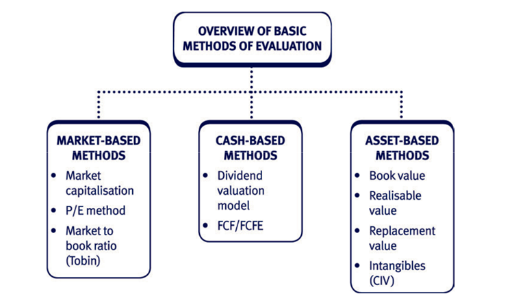
There are three basic ways of valuing a business:
- Cash based methods – the theoretical premise here is that the value of the company should be equal to the discounted value of future cash flows.
- Market based methods – where we assume that the market is efficient, so use market information (such as share prices and P/E ratios) for the target company and other companies. The assumption is that the market values businesses consistently so, if necessary, the value of one company can be used to find the value of another.
- Asset based methods – the firm’s assets form the basis for the company’s valuation. Asset based methods are difficult to apply to companies with high levels of intangible assets, but we shall look at methods of trying to value intangible as well as tangible assets.
We shall cover these methods in detail in the rest of this chapter.
Cash based methods
The free cash flow method
Free cash flows can used to find the value of a firm. This value can be used:
- to determine the price in a merger or acquisition
- to identify a share price for the sale of a block of shares
- to calculate the ‘shareholder value added’ (SVA) by management from one period to another.
Calculating the value
Technically, in order for the value of the business to be accurately determined, free cash flow for all future years should be estimated. However rather than attempting to predict the free cash flows for every year, in practice a short cut method is applied. Future cash flows are divided into two time periods:
- Those that occur during the ‘planning horizon’.
- Those that occur after the planning horizon.
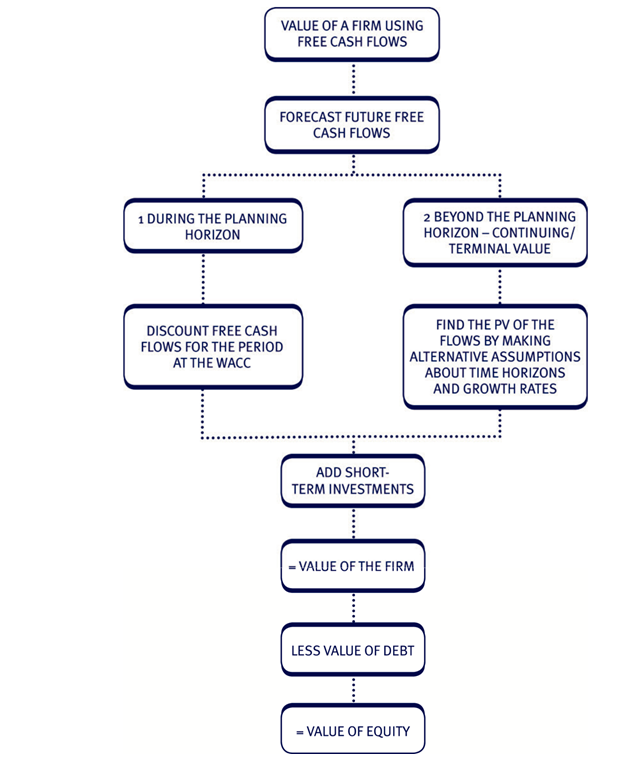
The planning horizon
The planning horizon is the period where:
- the firm can earn above average returns
- cash flows are assumed to grow over time.
Beyond the planning horizon, returns are expected to reach a steady state.
The planning horizon
In competitive industries, a business may have a period of ‘competitive advantage’ where it can earn excess returns on capital by maintaining a commercial advantage over the competition. However this period is unlikely to last indefinitely. Returns are likely to reach a steady state where the business earns on average its cost of capital but no more.
The planning horizon (which may last up to ten years or more) is the period during which the returns are expected to be higher than the cost of finance.
In period beyond the planning horizon it is usually assumed that the returns earned will continue at their current rate for the remainder of the investors’ time horizon. This may be a given number of years or in perpetuity. Alternatively the value of the cash flows may be expressed as a lump sum using a PE ratio.
Illustration 1
A company prepares a forecast of future free cash flow at the end of each year. A period of 15 years is used as this is thought to represent the typical time horizon of investors in this industry.
It is assumed that the planning horizon is three years – i.e. returns are likely to grow each year for the first three years after which they will reach a steady state.
The following data is available:
Free cash flows are expected to be $2.5 million in the first year, $4.5 million in the second year and $6.5 million in year 3. The stock market value of debt is $5m and the company’s cost of capital is 10%.
Required:
Calculate the current value of the firm and the value of the equity.
| Solution | ||||||
| Year 1 | Year 2 | Year 3 | Years 4–15 | |||
| Free cash flow | 2.5 | 4.5 | 6.5 | 6.5 | ||
| PV factor @ 10% | 0.909 | 0.826 | 0.751 | 6.814 × | ||
| 0.751 * | ||||||
| PV | 2.273 | 3.717 | 4.882 | 33.263 | ||
| Total PV = value of the firm | 44.135 | |||||
| Less value of debt | (5.000) | |||||
| Value of equity | 39.135 | |||||
| *12 year AF (gives T3 value of CF years 4 – 15) × 3 year DF (to discount | ||||||
| to T0). | ||||||
The valuation of debt
The value of debt was given in the previous illustration.
If you are not told the value in a question, the best way of estimating the value is by using the formula:
Value of debt = Present value of receipts to the lender (i.e. interest and redemption payment) discounted at the lender’s required rate of return
The valuation of debt is covered in more detail later in this chapter.
Further illustration
The company in the previous illustration now believes that earnings after the planning horizon will:
- continue at the year 3 level into perpetuity or
- grow at 0.9% pa into perpetuity.
Required:
Recalculate the current value of the firm and the value of the equity.
| Solution | ||||
| (a) | ||||
| Year 1 | Year 2 | Year 3 | Years 4 | |
| onwards | ||||
| Free cash flow | 2.5 | 4.5 | 6.5 | 6.5 |
| PV factor @ 10% | 0.909 | 0.826 | 0.751 | 1/0.1 × 0.751* |
| PV | 2.273 | 3.717 | 4.882 | 48.815 |
| Total PV = value of the firm | 59.687 | |||
| Less value of debt | (5.000) | |||
| Value of equity | 54.687 | |||
*1/i (gives T3 value of CF from year 4 onwards) × 3 year DF (to discount to T0).
Note the higher value that results when the time horizon is altered.
| (b) | ||||
| Year 1 | Year 2 | Year 3 | Years 4–infinity | |
| Free cash flow | 2.5 | 4.5 | 6.5 | 6.5 (infl 0.9%) |
| PV factor @ 10% | 0.909 | 0.826 | 0.751 | See working |
| PV | 2.273 | 3.717 | 4.882 | 54.126 |
Value of equity is 54.126 + 2.273 + 3.717 + 4.882 – (debt value) 5
- $59.998m Working:
The value of the growing perpetuity from Year 4 onwards can be calculated as:
[(6.5 × 1.009)/(0.10 – 0.009)] × 0.751 = 54.126
Calculating free cash flows from accounting information
When appraising an individual project in Chapter 2: Investment appraisal, the free cash flows could usually be estimated quite easily. However, identifying free cash flows for an entire company or business unit is much more complex, since there are potentially far more of them.
In these situations, the level of free cash flows is more usually determined from the already prepared accounting information and therefore is found by working back from profits as follows:
| Comment | ||
| Net operating profit (before | X | For future years, expected |
| interest and tax) | profits are predicted based on | |
| expected growth rates | ||
| Less taxation | (X) | A relevant cash flow and |
| therefore deducted from profit | ||
| Add depreciation | X | Not a cash flow and therefore |
| added back to profit | ||
| –––– | ||
| Operating cash flow | X | |
| Less investment: | ||
| Replacement non-current asset | (X) | Needed in order to continue |
| investment (RAI) | operations at current levels. If | |
| no information available about | ||
| amounts, it is assumed to be | ||
| equal to current levels of | ||
| depreciation | ||
| Incremental non-current asset | (X) | Needed to sustain expected |
| investment (IAI) | growth asset investment | |
| Incremental working capital | (X) | Needed to sustain expected |
| investment (IWCI) | growth | |
| –––– | ||
| Free cash flow | X | |
| –––– |
This method gives the level of free cash flow to the firm as a whole.
Free cash flow to equity
The above approach calculates free cash flows before deducting either interest or dividend payments.
The free cash flow to equity only can be calculated by taking the free cash flow calculated above and:
- deducting debt interest paid
- deducting any debt repayments
- adding any cash raised from debt issues.
In practical terms, the free cash flow to equity determines the dividend capacity of a firm i.e. the amount the firm can afford to pay out as a dividend.
More details on free cash flow
Cash that is not retained and then reinvested in a business is called free cash flow. This in effect represents the cash flow available to all the providers of capital of a company, whether these be debt holders or shareholders. This could be used to pay dividends or finance additional capital projects, if the necessary organisational criteria were met. Free cash flow is a very good measure of performance and an indicator of value.
Some would suggest that it is a better indicator of performance than measures based on net income. Forecast free cash flow is the most theoretically sound way to place a fair value on a company. Apparently Warren Buffet, the world’s richest investor, uses historic and forecast free cash flow to value the businesses that he buys.
Growing free cash flows are frequently a prelude to increased earnings and hence may be a positive sign for investors. Conversely a shrinking free cash flow may be an indicator of problems ahead, and a sign that companies are unable to sustain earnings growth. This may not always be the case, as many young companies put a lot of their cash into investments, which diminish their free cash flow. However, in this case questions might be raised about the sufficiency of short and long-term capital.
There can be variations in the definition. When calculating free cash flow over a number of years it is sensible to include the change in working capital and all investment spending. Over a long period of time the cash flow resulting from all investment is likely to be realised and so such a measure would be useful to those undertaking business valuations and using data forecast into the future.
However, when calculating free cash flow for a single year it would be sensible to omit the change in working capital and discretionary non-maintenance capital spending, because the ultimate payoff from those investments is not yet included in the operating cash flow. However, this in turn may give rise to debate about what represents the level of sustaining capital expenditure that should be deducted. When analysing figures for free cash flow it is also important to be aware of any unusual events in a particular year, which may impact on the cash flow.
Figures calculated for free cash flow can be used in determining a company’s cash flow ratios.
For example:
Dividend cover in cash terms = Free cash flow to equity/Dividends paid
It is argued that this measure of dividend cover is better than the conventional ratio of earnings divided by dividends paid, since dividends are paid in cash, and with no cash there can’t be any dividends.
Also, since the free cash flow to equity determines the company’s dividend capacity (explained in detail in Chapter 5: The dividend decision) we can see from the breakdown of free cash flow to equity that there is a strong link between new investments and dividend capacity i.e. if a new investment project increases the cash inflows of a business, its free cash flow to equity and hence its dividend capacity will increase.
Illustration of calculations of free cash flow
Calculate the free cash flow based on the following figures:
(a) using the standard approach
| (b) to show the free cash flow to equity. | |
| $000 | |
| Operating profit | 300 |
| Depreciation | 120 |
| Increase in working capital | 50 |
| Capital expenditure to replace existing assets | 10 |
| Capital expenditure on new investments | 15 |
| Interest paid | 5 |
| Loans repaid | 20 |
| Tax paid | 140 |
| Solution | |
| (a) Standard approach | |
| $000 | |
| Net operating profit (before interest and tax) | 300 |
| Plus depreciation | 120 |
| Less taxation | (140) |
| –––– | |
| Operating cash flow | 280 |
| Less investment: | |
| Replacement non-current asset investment | (10) |
| Incremental non-current asset investment | (15) |
| Incremental working capital investment | (50) |
| –––– | |
| Free cash flow | 205 |
| –––– | |
| (b) Free cash flow to equity | |
| $000 | |
| Free cash flow to the firm | 205 |
| Less debt interest paid | (5) |
| Less loans repaid | (20) |
| –––– | |
| Free cash flows to equity | 180 |
| –––– | |
Forecasting growth in free cash flows
The methods above have identified a figure for the free cash flow of the business based on its current financial statements. In order to value the business, the future free cash flows need to be forecast and then discounted.
To forecast the likely growth rate for the free cash flows, the following three methods can be used:
Historical estimates
For example, if the business has achieved growth of 5% per annum each year for the last five years, 5% may be a sensible growth rate to apply to future free cash flows.
Analyst forecasts
Particularly for listed companies, market analysts regularly produce forecasts of growth. These independent estimates could be a useful indicator of the likely future growth rate.
Fundamental analysis
The formula for Gordon’s growth approximation (g = r × b) can be used to calculate the likely future growth rate, where r is the company’s return on equity (cost of equity) and b is the earnings retention rate. The formula is based on the assumption that growth will be driven by the reinvestment of earnings.
Alternatively, in an exam question, you may simply be told which growth rate to apply.
Use of free cash flow to equity (FCFE) in valuation
The previous calculations have found equity value by:
- discounting free cash flow to present value using the WACC, and then deducting debt value. This is known as the free cash flow to firm methodology.
Alternatively, the value of equity can be found directly by:
- discounting free cash flow TO EQUITY at the cost of equity.
In the simplest case (if FCFE is assumed to be growing at a constant rate into perpetuity), the following formula can be applied:
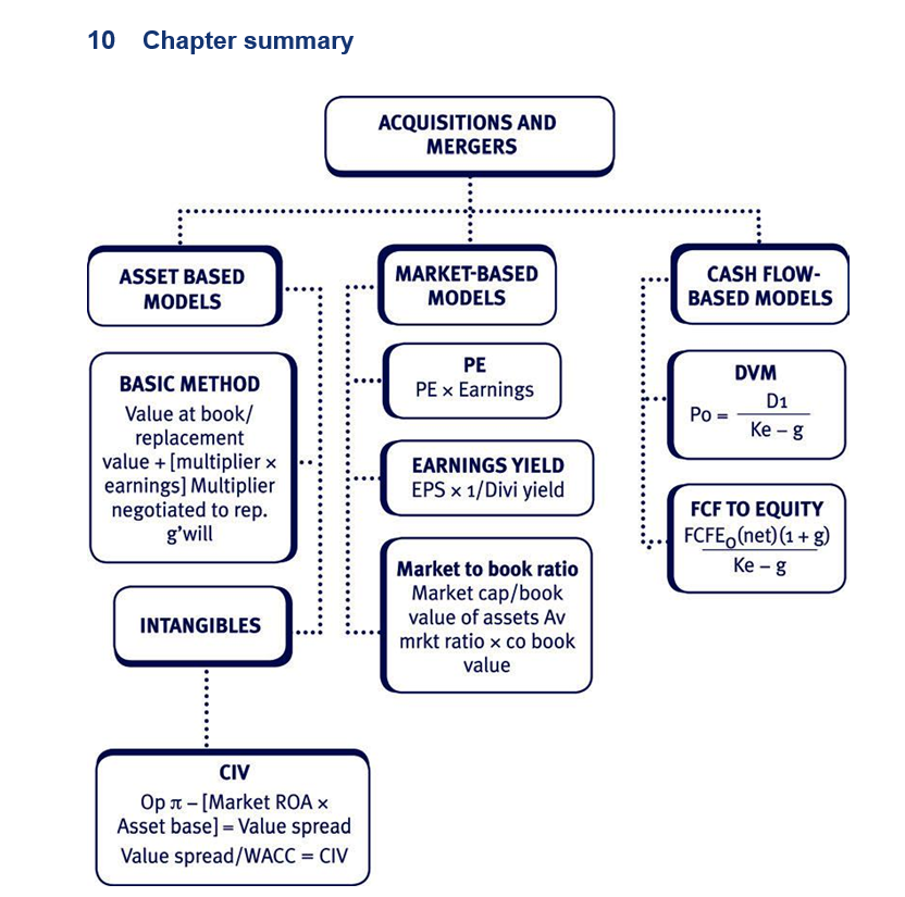
FCFE0(1 + g)/(ke – g)
The formula is based on the dividend valuation model theory (see below for more details on using DVM in business valuation).
The dividend valuation model (DVM)
Theory: The value of the share is the present value of the expected future dividends discounted at the shareholders’ required rate of return.
Assuming a constant growth rate in dividends, g:
P0 = D0(1 + g)/(ke – g)
Note that:
If D0 = Total dividends P0 = Total value of the company’s equity.
If D0 = Dividends per share P0 = Value per share.
If the growth pattern of dividends is not expected to be stable, but will vary over time, the formula can be adapted.
Explanation of terms in DVM formula
Ke = cost of equity.
g = constant rate of growth in dividends, expressed as a decimal.
D0(1 + g) = dividend just paid adjusted for one year’s growth.
DVM calculations
Basic application of DVM formula
A company has just paid a dividend of 20¢. The company expects dividends to grow at 7% in the future. The company’s current cost of equity is 12%.
Required:
Calculate the market value of the share.
Solution
P0 = 20(1 + 0.07)/(0.12 – 0.07) = 428¢ = $4.28
More advanced application of the DVM formula
C plc has just paid a dividend of 25¢ per share. The return on equities in this risk class is 20%.
Required:
Calculate the value of the shares assuming:
- no growth in dividends
- constant growth of 5% pa
- constant dividends for 5 years and then growth of 5% pa to perpetuity.
Solution
- P0 = 0.25/0.2 = $1.25
- P0 = 0.25(1.05)/(0.2 – 0.05) = $1.75
- Present value of first
5 years’ dividends = 0.25 × 5 yr 20% AF 0.748
| = | 0.25 × 2.991 | ||
| Present value of growing | |||
| dividend | = | Value at T5 × 5 yr DF | |
| = | [0.25(1.05)/ | ||
| (0.2 – 0.05)] × 0.402 | 0.704 | ||
| –––––– | |||
| Share value | $1.452 | ||
| –––––– |
Test your understanding 3
C plc has just paid a dividend of 32 cents per share. The return on equities in this risk class is 16%.
Required:
Calculate the value of each share, assuming constant dividends for 3 years and then growth of 4% pa to perpetuity.
The model is highly sensitive to changes in assumptions:
- Where growth is high relative to the shareholders’ required return, the share price is very volatile.
- Even a minor change in investors’ expectations of growth rates can cause a major change in share price contributing to the share price crashes seen in recent years.
Illustration of sensitivity of DVM
Consider the impact of a change in growth predictions of 0.5% in two cases – the first where growth is low compared to the firm’s required return, the other where it is high.
A firm’s ke is 7% and D0 is 10 cents.
The change in share price as a result of changing growth predictions is shown.
Assuming:
- a growth rate of 2% dropping to 1.5%
- a growth rate of 5% dropping to 4.5%.
Assumption (i)
Share price at g = 2% 10 × 1.02/(0.07 – 0.02) = 204
Share price at g = 1.5% 10 × 1.015/(0.07 – 0.015) = 184.55 Fall in share price is (204 – 184.55)/204 = 9.5%
Assumption (ii)
Share price at g = 5% 10 × 1.05/(0.07 – 0.05) = 525
Share price at g = 4.5% 10 × 1.045/(0.07 – 0.045) = 418
Fall in share price is (525 – 418)/525 = 20.4%
The share price shows far greater volatility where growth is high relative to required return.
DVM is more suitable for valuing minority stakes, since it only considers dividends. In practice the model does tend to accurately match actual stock market share prices.
4 Market based methods
Stock market value (market capitalisation)
For a listed company, the stock market value of the shares (or ‘market capitalisation’) is the starting point for the valuation process.
In a perfectly efficient market, the market price of the shares would be fair at all times, and would accurately reflect all information about a company. In reality, share prices tend to reflect publicly available information.
The market share price is suitable when purchasing a minority stake. However, a premium usually has to be paid above the current market price in order to acquire a controlling interest.
The price-earnings ratio (P/E) method
The P/E method is a very simple method of valuation. It is the most commonly used method in practice.
P/E valuation method formula
Value per share = EPS × P/E ratio
Total equity value of the company = Total post-tax earnings × P/E ratio
Using the P/E valuation formula
The P/E ratio method is the simplest valuation method. It relies on just two figures (the post-tax earnings and the P/E ratio).
Post-tax earnings
The current post -tax earnings, or EPS, for a company can easily be found by looking at the most recent published accounts. However, these published figures will be historic, whereas the earnings figure needed for valuation purposes should be an expected, future earnings figure.
It is perfectly acceptable to use the published earnings figure as a starting point, but before performing the valuation, the historic earnings figure should be adjusted for factors such as:
- one-off items which will not recur in the coming year (e.g. debt write offs in the previous year)
- directors’ salaries which might be adjusted after a takeover has been completed
- any savings (‘synergies’) which might be made as part of a takeover.
P/E ratio
The P/E ratio for a listed company is a simple measure of the company’s share price divided by its earnings per share.
The P/E indicates the market’s perception of the company’s current position and its future prospects. For example, if the P/E ratio is high, this indicates that the company has a relatively high share price compared to its current level of earnings, suggesting that the share price reflects good growth prospects of the company.
An unlisted company has no market share price, so has no readily available P/E ratio. Therefore, when valuing an unlisted company, a proxy P/E ratio from a similar listed company is often used.
Proxy P/E ratios
As explained above, an unlisted company will not have a market-driven P/E ratio, so an industry average P/E, or one for a similar company, will be used as a proxy.
However, proxy P/E ratios are also sometimes used when valuing a listed company – of course if a listed entity’s own P/E ratio is applied to its own earnings figure, the calculation will just give the existing share price.
Test your understanding 4
Molier is an unquoted entity with a recently reported after-tax earnings of $3,840,000. It has issued 1 m ordinary shares. A similar listed entity has a P/E ratio of 9.
Required:
Calculate the value of one ordinary share in Molier using the P/E basis of valuation.
The strengths and weaknesses of P/E valuations
The main strengths of P/E valuations are:
- they are commonly used and are well understood
- they are relevant for valuing a controlling interest in an entity. The main weaknesses of P/E valuations are:
- they are based on accounting profits rather than cash flows
- it is difficult to identify a suitable P/E ratio, particularly when valuing the shares of an unlisted entity
- it is difficult to establish the relevant level of sustainable earnings.
Test your understanding 5
ABC Co is considering making a bid for the entire equity capital of XYZ Co, a firm which has a PE ratio of 9 and annual earnings of $390m.
ABC Co has a PE of 13 and annual earnings of $693m, and it is thought that $ 125m of annual synergistic savings will be made as a consequence of the takeover. The PE of the combined company is expected to be 12.
Required:
Calculate the minimum value acceptable to XYZ’s shareholders, and the maximum amount which ABC should consider paying.
Earnings yield method
In some questions, you may not be given the P/E ratio, but you may be given the Earnings Yield instead.
The earnings yield is the reciprocal of the P/E ratio i.e. Earnings Yield = 1 /(P/E ratio). Hence
Value of company = Total earnings/Earnings Yield
Value per share = EPS/Earnings Yield
Understanding and interpretation of earnings yield
Some deeper analysis is desirable, for example examining the trend of share price over a number of quarters in the light of any events such as profits warnings and acquisitions (or rumours thereof), and the likely effect that they have had on earnings.
The stability of Earnings Yield is often as important as its growth, bearing in mind that in a general way the market is absorbing new information to try to assess a sustainable level of EPS on which to base growth for the future. Clearly, effective growth is dependent on a stable base, and the trend of Earnings Yield over time is to an extent a reflection of this factor.
A prospective acquirer would, of course, be concerned to assess the worth of a prospective target on the basis of its becoming part of the acquiring entity, and the valuation will especially need to take into account the expectations of the target’s shareholders.
Tobin’s market to book ratio
Market to book ratio (based on Tobin’s Q)
Market value of target company = Market to book ratio × book value of target company’s assets
where market to book ratio = (Market capitalisation/Book value of assets)
for a comparator company (or take industry average)
This method assumes a constant relationship between market value of the equity and the book value of the firm.
Problems with the model:
- Choosing an appropriate comparator – should we use industry average, or an average of similar firms only?
- The ratio the market applies is not constant throughout its business cycle, so strictly the comparator should be taken only from other companies at the same stage.
Illustration of Tobin’s Q
The industry sector average Market to Book ratio for the industry of X plc is 4.024.
The book value of X plc is $3,706m and it has 1,500m shares in issue.
Required:
Calculate the predicted share price.
Solution
Predicted value of X plc = $3,706m × 4.024 = $14,912.94m.
Predicted share price = $14,912.94m/1,500m = 994.2¢.
Asset based methods
The basic model
The traditional asset based valuation method is to take as a starting point the value of all the firm’s statement of financial position assets less any liabilities. Asset values used can be:
- book value – the book value of assets can easily be found from the financial statements. However, it is unlikely that book values (which are based on historic cost accounting principles) will be a reliable indicator of current market values.
- replacement cost – the buyer of a business will be interested in the replacement cost, since this represents the alternative cost of setting up a similar business from scratch (organic growth versus acquisition).
- net realisable value – the seller of a business will usually see the realisable value of assets as the minimum acceptable price in negotiations.
However:
- replacement cost is not easy to identify in practice, and
- the business is more than just the sum of its constituent parts. In fact the value of the tangible assets in many businesses is minimal since much of the value comes from the intangible assets and goodwill (e.g. compare a firm of accountants with a mining company).
Intangible asset valuation methods
Definition of intangible assets
Intangible assets are those assets that cannot be touched, weighed or physically measured. They include:
- assets such as patents with legal rights attached
- intangibles such as goodwill, purchased and valued as part of a previous acquisition
- relationships, networks and skills built up by the business over time.
A major flaw with the basic asset valuation model is that it does not take account of the true value of intangibles.
Basic intangible valuation method
The simplest way of incorporating intangible value into the process is by the following basic formula:
Firm value = [book or replacement cost of the real assets] + [multiplier × annual profit or revenue]
The multiplier is negotiated between the parties to compensate for goodwill.
Effectively, some attempt is being made to estimate the extra value generated by the intangible assets, above the value of the firm’s tangible assets.
This simple formula provides the basis for the two main intangible valuation methods: CIV (Calculated Intangible Value) and Lev’s method.
More detail on intangible assets
Often intangible assets, making up a significant part of the real worth of the company, are formed by the staff of a company – their skills, knowledge and creativity. Such assets are created by spending on areas such as R&D, advertising and marketing, training and staff development. This type of expenditure serves to enhance the underlying value of the firm rather than assisting directly in earning this year’s profits.
A significant problem with the basic asset valuation model is that the assets to be valued are taken to be those identified on the statement of financial position. Where a firm has significant levels of intangible assets, accounting conventions mean they will be either not be included at all, or included at amounts well below their real commercial value.
If the asset based model is to be of use, a way of valuing these intangibles must be found.
Calculated intangible value (CIV)
This method is based on comparing (benchmarking) the return on assets earned by the company with:
- a similar company in the same industry or
- the industry average.
The method is similar to the residual income technique you may remember from your earlier studies. It calculates the company’s value spread – the profit it earns over the return on assets that would be expected for a firm in that business.
Method
- A suitable competitor (similar in size, structure etc.) is identified and their return on assets calculated:
Operating profit/Assets employed
- If no suitable similar competitor can be identified, the industry average return may be used.
- The company’s value spread is then calculated.
| $ | |
| Company operating profit | X |
| Less: | |
| Appropriate ROA × Company asset base | (X) |
| ––– | |
| Value spread | X |
| ––– |
- Assuming that the value spread would be earned in perpetuity, the Calculated Intangible Value (CIV) is found as follows:
– Find the post-tax value spread.
– Divide the post-tax value spread by the cost of capital to find the present value of the post-tax value spread as a perpetuity (the CIV).
- The CIV is added to the net asset value to give an overall value of the firm.
CIV calculation
CXM operates in the advertising industry. The directors are keen to value the company for the purposes of negotiating with a potential purchaser and plan to use the CIV method to value the intangible element.
In the past year CXM made an operating profit of $137.4 million on an asset base of $307 million. The company WACC is 6.5%.
A suitable competitor for benchmarking has been identified as R. R made an operating profit of $315 million on assets employed in the business of $1,583 million.
Corporation tax is 30%.
Required:
Calculate the value of CXM, including the CIV.
Solution
- R is currently earning a return of 315/1,583 = 19.9%
- The value spread for CXM is:
| $m | |
| Company operating profit | 137.40 |
| Less | |
| Appropriate ROA × Company asset base (19.9% × | |
| 307) | 61.09 |
| –––––– | |
| Value spread | 76.31 |
| –––––– |
- Calculate the CIV:
– Find the post-tax value spread $76.31 × (1 – 0.3) = 53.42
– Find the CIV by calculating the PV of the post-tax value spread (assuming it will continue into perpetuity)
CIV = 53.42/0.065 = $822m
- The overall value of the firm = CIV + asset base Firm value = $822m + $307m = $1,129m.
Problems with the CIV model:
- Finding a similar company in terms of industry, similar asset portfolio, similar cost gearing etc.
- Since the competitor firm presumably also has intangibles, CIV actually measures the surplus intangible value our company has over that of the competitor rather than over its own asset value.
Lev’s knowledge earnings method
An alternative method of valuing intangible assets involves isolating the earnings deemed to be related to intangible assets, and capitalising them. However it is more complex than the CIV model in how it determines the return to intangibles and the future growth assumptions made.
In practice, this model does produce results that are close to the actual traded share price, suggesting that is a good valuation technique.
However, it is often criticised as over complex given that valuations are in the end dependent on negotiation between the parties.
Risk in acquisitions and mergers
An acquisition may expose an acquiring company to risk. It is important to distinguish between:
- business risk
- financial risk.
Business risk
This is the variability in the earnings of the company, which results from the uncertainties in the business environment. If the merger or acquisition is with another company operating in the same business area, the underlying business risk (measured by the asset beta) of the acquirer will be unaffected.
Financial risk
Financial risk is the additional volatility caused by the firm’s gearing structure. If an acquisition is significant in size relative to the acquirer or requires an alteration to the firm’s capital structure, it will change the acquirer’s exposure to finance risk.
Valuation and risk
It is a key principle that the most an acquirer should ever pay for a target company is the increase in the value of the acquiring firm arising from the acquisition.
However, it is rarely a simple matter of valuing the target and assuming that will be the level of increase experienced. This ignores the impact of:
- potential synergy gains – although there is an argument that they are so rarely achieved in practice that they should be very conservatively estimated, and only then if they are arising because of the target itself (that is they wouldn’t arise from any merger)
- the change in potential risk profile of the combined entity as discussed above.
The valuation techniques used must therefore depend on the type of acquisition being considered.
For example, if an NPV based approach is being used for valuation, a risk adjusted cost of capital (appropriate to the risk of the cash flows being considered) may need to be calculated and used for discounting.
In fact, the methods introduced in the earlier Chapter 7: Risk adjusted WACC and adjusted present value are equally relevant in business valuation. So the risk adjusted WACC can be used as a discount rate when dealing with a change in business risk and/or a small change in financial risk, whereas the APV method can be used when there is a significant change in capital structure. Some examples of these approaches are shown below.
Similarly, if a price-earnings (P/E) valuation method is being used, the proxy P/E ratio used in the calculation must reflect the risk profile and growth prospects of the company’s earnings being valued.
Worked example using risk adjusted WACC in valuation
A risk adjusted WACC approach is often used when discounting the expected cash flows of the combined company after an acquisition or merger.
Overview of method
Step 1: Calculate the asset beta of both companies before the acquisition.
Step 2: Calculate the average asset beta for the new combined company after the acquisition.
Step 3: Regear this beta to reflect the post-acquisition gearing of the new combined company.
Step 4: Calculate the combined company’s WACC.
Step 5: Discount the post-acquisition free cash flows using this WACC.
Step 6: Calculate the NPV and deduct the value of debt to give the combined company’s value of equity.
A worked example using this method follows.
Worked example
Anderson Co is planning to take over Webb Co, a company in a different business sector, with a different level of risk. Anderson Co’s free cash flows are forecast to be $50m per annum in perpetuity, Webb Co’s free cash flows are forecast to be $10m per annum into perpetuity and there are expected to be annual post-tax cash synergies of $5m if the acquisition goes ahead.
The combined company will pay tax at 30% and will have a pre-tax cost of debt of 5%. The risk free rate is 3% and the equity risk premium is 5.8%.
Currently, Anderson Co has an asset beta of 1.25 and Webb Co has an asset beta of 1.60. Assume that the beta of debt is zero.
| The current financing of the two companies is: | ||
| $million | Debt | Equity |
| Anderson Co | 50 | 450 |
| Webb Co | 20 | 80 |
Anderson Co is planning to make a cash offer of $80m to buy 100% of the shares of Webb Co. The cash offer will be funded by additional borrowing.
Required:
Calculate the gain in wealth for Anderson Co’s shareholders if the acquisition goes ahead.
Solution
The asset beta of the combined company is (1.25 × (500/600)) + (1.60 × (100/600)) = 1.31
Therefore, the equity beta of the combined company is (using the asset beta formula from the formula sheet and assuming the new gearing is
150 debt to 530 equity):
1.31 × (1 + [0.7 × (150/530)]) = 1.57
Hence, using CAPM, the cost of equity is: 3% + (1.57 × 5.8%) = 12.1%
and so the WACC = (12.1% × (530/680)) + (5% × (1 – 0.30%) × (150/680)) = 10.2%
Therefore, the discounted free cash flows of the combined company are (as a perpetuity):
($50m + $10m + $5m)/0.102 = $637m.
The value of equity is then this NPV – the value of debt, i.e.
$637m – $150m = $487m
Hence the shareholder wealth of the Anderson Co shareholders has increased from $450m to $487m as a consequence of the acquisition.
Worked example using APV in valuation
In the earlier Chapter 7: Risk adjusted WACC and adjusted present value (APV), we saw that the APV method can be used to appraise a project when there is a significant change in financial risk (capital structure).
The application of the APV method to valuation
In the context of project appraisal, the APV was found by discounting the project cash flows at the ungeared cost of equity, and then adjusting for the costs and benefits associated with the actual financing used.
The approach used in valuation is very similar. In fact, to value a target company using APV, the method is:
- calculate the present value of the target’s free cash flows, using the ungeared cost of equity as a discount rate
- add the present value of the tax saved as a result of the debt finance used in the acquisition (using either the risk free rate or the pre-tax cost of debt as a discount rate)
- find the value of the target’s equity (by deducting the value of the target’s debt from the value calculated in step 2 above).
Then this value of the target’s equity can be compared with the proposed acquisition cost to assess whether the acquisition should proceed.
Worked example
Derman Co is considering the acquisition of Weaver Co, an unquoted company. The shareholders of Weaver Co are hoping to receive $75 million for the sale of their shares.
The ungeared (asset) beta factor for Weaver Co is 1.20, the risk free rate of interest is 3% and the market risk premium is 5.8%.
Forecast free cash flows for Weaver Co are as follows:
$ million
Year 1
Year 2
Year 3
Year 4
Free Cash Flow
10.3 11.5 13.8 14.9
Annual cash flows after year 4 are expected to stay constant into perpetuity.
Weaver Co has $50 million of 6% debt, repayable in 4 years. The tax rate is 30%.
Required:
Using the APV method of valuation, calculate whether Derman Co should be prepared to pay the $75 million required by the shareholders of Weaver Co.
| Solution | ||||
| $ million | Year 1 | Year 2 | Year 3 | Year 4 etc |
| Free cash flow | 10.3 | 11.5 | 13.8 | 14.9 |
| DF at 10% (see W1) | 0.909 | 0.826 | 0.751 | (1/0.10) × 0.751 |
| PV | 9.36 | 9.50 | 10.36 | 111.90 |
NPV = $141.12 million
(W1) CAPM: Ungeared cost of equity = 3% + (1.20 × 5.8%) = 9.96%, say
10%.
PV of tax relief on debt interest:
The interest paid will be 6% × $50 million = $3 million from year 1 to year 4.
Therefore, tax relief is 30% × $3 million = $0.9 million per year
Discounted at 6% (the pre-tax cost of debt) this has a present value of:
$0.9m × Annuity factor for 4 years at 6%
= $0.9m × 3.465 = $3.12 million
APV
So the total APV is $141.12m + $3.12m = $144.24 million
Thus, the equity value of Weaver Co is $144.24m – $50m = $94.24 million.
This is significantly more than the $75 million that the shareholders are hoping for, so Derman Co should pay the $75 million and take over Weaver Co.
Student Accountant article
The article ‘Business valuations’ in the Technical Articles section of the ACCA website provides further details on the various valuation methods shown in this chapter.
7 The valuation of debt
Introduction
Throughout this chapter so far, we have been calculating a value for the equity of a business, on the basis that on an acquisition, the acquirer has to purchase the equity (or certainly a controlling share of it). Therefore, equity valuation is a critical issue in every acquisition.
The value of the debt in a company is often quite easy to determine, and not as subjective as the value of equity. For example, a bank loan is not traded so its value doesn’t fluctuate. However, traded debt (such as bonds) will have a fluctuating value so it is important that we can calculate a theoretical value for such debt.
Basic debt valuation model
The basic model for valuing a bond (or indeed any other type of debt) is similar to the cash based valuation methods discussed earlier i.e. the value of the bond will be the present value of the expected future receipts from the bond, discounted at the lender’s required rate of return.
In this case, the receipts to the investor are the interest payments and the redemption amount from the bond.
Illustration 2 – Basic debt valuation
Frank Co has some $100 nominal value, 6% coupon bonds in issue. The bonds are redeemable at par in 5 years and investors require a return of 4% from investments of this level of risk.
Required:
Calculate the value of each Frank Co bond.
Solution
PV of receipts = ($6 × annuity factor for 5 years at 4%) + ($100 × discount factor for 5 years at 4%)
= (6 × 4.452) + (100 × 0.822) = $108.91
Estimating the required return to the debt holder
In the example above, the calculations were simple because we knew what the required return of the debt holder was. However, we saw in the earlier chapter on the weighted average cost of capital that the required return of the debt holder (sometimes called the ‘yield’ on the debt) is not always easy to estimate. In this earlier chapter, we saw how to derive the yield by either:
- adding a given credit spread onto the risk free rate, or
- deriving a yield curve for bonds with different redemption dates.
Therefore, exam questions might well link these two parts of the syllabus together i.e. you might first have to derive the yield on a bond, as seen in the earlier chapter on the weighted average cost of capital, and then use the yield as a discount rate to calculate the bond’s value.
Illustration 3 – Use of credit spreads
Paper Co has some 5 year bonds in issue. It is an A rated company according to the main credit rating agencies.
The risk free rate of interest is 2.5%.
The current table of credit spreads (in basis points) published by one of the main agencies gives the following information:
| Rating | 1 yr | 3 yr | 5 yr | 10 yr | 20 yr |
| AAA | 12 | 25 | 60 | 100 | 150 |
| AA | 19 | 40 | 80 | 150 | 211 |
| A | 28 | 56 | 99 | 221 | 276 |
Therefore, the yield on Paper Co’s five year bonds can be found by adding the relevant credit spread to the risk free rate.
i.e. 2.5% + 99 basis points = 3.49%
The value of Paper Co’s bonds can now be calculated by discounting future interest and redemption payments at this 3.49%.
Illustration 4 – Use of the yield curve
Stone Co is about to issue some 3 year, $100 par value, 5% coupon bonds.
The issue price (bond value) should be calculated by discounting each year’s forecast cash flow from the bond at the relevant rate from the yield curve.
For Stone Co, assume the yield curve is:
| Year | Individual yield curve (%) |
| 1 | 3.96 |
| 2 | 4.25 |
| 3 | 4.56 |
Therefore, these 3 year, 5% coupon bonds should be issued at:
($5/1.0396) + ($5/1.04252) + ($105/1.04563)
= $101.26 (per $100 par value).
Student Accountant article
The examiner’s article ‘Bond valuation and bond yields’ in the Technical Articles section of the ACCA website covers the calculation of bond yield curves and values in more detail.
High growth start-ups
A start-up business that wishes to attract equity investment will need to put a value on the business.
Valuing start-up businesses presents a different challenge from valuing an existing business, because unlike well-established firms many start-ups have:
- little or no track record
- ongoing losses
- few concrete revenues
- unknown or untested products
- little market presence.
In addition, they are often staffed by inexperienced managers with unrealistic expectations of future profitability and the lack of past data makes prediction of future cash flows extremely difficult.
Any mathematical valuation will inevitably be only an early starting point in the negotiations.
More detail on valuation of start-up businesses
Estimating growth
Growth for a start-up can be estimated based on:
- industry projections from securities analysts
- qualitative evaluation of the company’s management, marketing strengths and level of investment.
However, both of these are essentially subjective and are unlikely to be reliable.
Since high-growth start-ups usually cannot fund operating expenses and investment needs out of revenues, long-term financial projections will be essential.
High growth is one thing, profitable high growth is another.
Growth in operating income is a function of:
- management’s investment decisions:
– How much a company reinvests.
– The effectiveness of the investment in achieving results.
- the markets acceptance of the product and the action of competitors
- management’s skills
- the riskiness of the industry.
Valuation methods
Since the estimate of growth is so unpredictable and initial high growth can so easily stagnate or decline, valuation methods that rely on growth estimates are of little value:
- Cash is key indicator of start-up success and asset models are therefore an important starting point.
However, they cannot provide an accurate value, since value rests more on potential than on the assets in place:
- DCF models are problematic because of the non-linear and unpredictable performance often exhibited in the early years, rendering the estimates highly speculative.
- Market based models are difficult to apply because of the problem of finding similar companies to provide a basis for comparison.
9 Problems of overvaluation
A share is overvalued if it is trading at a price that is higher than its underlying value.
In an efficient market this can still occur if:
- the market doesn’t properly understand the business (as with internet businesses in the late 1990s) and overestimates the expected returns
- the managers running the company do not convey full company information honestly and accurately.
Management responses to overvaluation
Managers may be reluctant to correct the markets’ mistaken perceptions. This can lead to:
- the use of creative accounting to produce the results the city is expecting
- poor business decisions aimed at giving the impression of success
- ‘poor’ acquisitions made using inflated equity to finance the purchase.
The impact of overvaluation on reported earnings
Since managers may manipulate reported earnings to produce more favourable results, the financial data they supply should be treated with caution. When valuing a company the financial statements should first be analysed and adjusted as necessary.
Why firms may be overvalued
Empirical evidence suggests that stock markets are semi-strong efficient
– i.e. equity prices reflect all publicly available information. However, this does not necessarily mean that the shares will be fairly valued:
- If the market doesn’t fully understand the information available – as was the case in the late 1990s and early 2000s with some high-tech, telecommunications, and internet ventures – it tends to overestimate the potential returns and so overvalue the equity.
- The price of overvalued equity may not be corrected by the market if:
– the data provided by managers is deliberately misleading; a particular problem where the agency relationships within companies breaks down
– there is collusion by gatekeepers including investment and commercial banks, and audit and law firms (many of whom have been accused of knowingly contributing to the misinformation and manipulation that fed the overvaluation of stocks such as Enron and Worldcom amongst others).
The response of management
When a firm produces earnings that beat analysts’ forecasts, the share price rises by 5.5% on average. For unexpected negative earnings, the share price falls on average by 5.05%. Even where shares are fairly priced shares, managers may hide the inherent uncertainty in the business by smoothing earnings figures – delaying expenses and bringing forward revenue recognition, for example to ensure they consistently meet investor expectations.
If equity remains overpriced, the company will not be able to deliver – except by pure luck – the performance to justify its value. Where the management of an overvalued company is unwilling to accept the pain of a stock market correction, earnings smoothing can escalate into false accounting and outright lying. In addition, projects that give the appearance of potential earnings may be adopted even where the true likely outcome is a negative NPV, in order to forestall city concerns.
Research has also shown that companies are more likely to make acquisitions when their shares are overvalued. This is because they can use the shares to buy assets (which have true worth). However, these mergers often do not make good business sense and can destroy the core value of the firm.
Case study
At the time of Enron’s peak market value of $60 billion, the company was worth about 70 times its earnings and 6 times its book value of assets. The company was a major innovator, and the business had a viable future. However, senior managers were unwilling to see the excess valuation diminished. Rather than communicate honestly with the market to reduce its expectations, they tried to hide the overvaluation by manipulating the financial statements and exaggerating the value of new ventures. By the time the market had realised the extent of the problem, the core value of the company had been destroyed.
Implications for valuations
In valuing a company, reported results form an essential core of data. Since reported earnings may be manipulated to produce more favourable results (aggressive accounting) the financial statements should be scrutinised and restated as necessary before being used as the basis for any valuation.
The detailed techniques are outside the syllabus but would include:
- Calculating the Cash to Operating Profit (COP) ratio. This involves comparing EBITDA (Earnings before Interest, Tax, Depreciation and Amortisation) with operating cash flow – they should be about equal. A figure above one is an indicator of aggressive accounting.
- Adjusting for changes in:
– depreciation/amortisation policy
– bad debt provisions.
- Considering whether the amortisation of intangibles and R&D is appropriate and adjusting if necessary.
- Making changes if necessary to the way leases and hire purchase agreements have been accounted for:
– Removing any exceptional items.
– Removing any exceptional payments such as directors’ severance payments.
One thought on “Business valuation”