
Most financial decisions, such as the purchase of assets or procurement of funds, affect the firm’s cash flows in different time periods. For example, if a fixed asset is purchased, it will require an immediate cash outlay and will generate cash inflows during many future periods. Similarly, if the firm borrows funds from a bank or from any other source, it receives cash now and commits an obligation to pay cash for interest and repay principal in future periods. The firm may also raise funds by issuing equity shares. The firm’s cash balance will increase at the time shares are issued, but, as the firm pays dividends in future, the outflow of cash will occur. Sound decision making requires that the cash flows, which a firm is expected to receive or give up over a period of time, should be logically comparable. In fact, the absolute cash flows, which differ in timing and risk, are not directly comparable. Cash flows become logically comparable when they are appropriately adjusted for their differences in timing and risk.
The recognition of the time value of money and risk is extremely vital in financial decision making. If the timing and risk of cash flows is not considered, the firm may make decisions that may allow it to miss its objective of maximizing the owners’ welfare. The welfare of owners would be maximized when wealth or net present value is created from making a financial decision. What is net present value? How is it computed?
TIME PREFERENCE FOR MONEY
Three reasons may be attributed to the individual’s time preference for money:1 risk
If an individual behaves rationally, he or she would not value the opportunity to receive a specific amount of money now, equally with the opportunity to have the same amount at some future date. Most individuals value the opportunity to receive money now higher than waiting for one or more periods to receive the same amount. Time preference for money or Time Value of Money (TVM) is an individual’s preference for possession of a given amount of money now, rather than the same amount at some future time.
preference for consumption investment opportunities
We live under risk or uncertainty.* As an individual is not certain about future cash receipts, he or she prefers receiving cash now. Most people have subjective preference for present consumption over future consumption of goods and services either because of the urgency of their present wants or because of the risk of not being in a position to enjoy future consumption that may be caused by illness or death, or because of inflation. As money is the means by which individuals acquire most goods and services, they may prefer to have money now. Further, most individuals prefer present cash to future cash because of the available investment opportunities to which they can put present cash to earn additional cash. For example, an individual who is offered `100 now or `100 one year from now would prefer `100 now as he could earn on it an interest of, say, `5 by putting it in the savings account in a bank for one year. His total cash inflow in one year from now will be `105. Thus, if he wishes to increase his cash resources, the opportunity to earn interest would lead him to prefer `100 now, not `100 after one year.
In case of the firms as well, the justification for time preference for money lies simply in the availability of investment opportunities.2 In financial decision making under certainty, the firm has to determine whether one alternative yields more cash or the other. In case of a firm, which is owned by a large number of individuals (shareholders), it is neither needed
nor is it possible to consider the consumption preferences of owners. The uncertainty about future cash flows is also not a sufficient justification for time preference for money. We are not certain even about the usefulness of the present cash held; it may be lost or stolen. In investment and other decisions of the firm what is needed is the search for methods of improving decision maker’s knowledge about the future. In the firm’s investment decision, for example, certain statistical tools such as probability theory, or decision tree could be used to handle the uncertainty associated with cash flows.
Required Rate of Return
The time preference for money is generally expressed by an interest rate. This rate will be positive even in the absence of any risk. It may therefore be called the risk-free rate. For instance, if time preference rate is 5 per cent, it implies that an investor can forego the opportunity of receiving `100 if he is offered `105 after one year (i.e., `100 which he would have received now plus the interest which he could earn in a year by investing `100 at 5 per cent). Thus, the individual is indifferent between `100 and `105 a year from now as he considers these two amounts equivalent in value. In reality, an investor will be exposed to some degree of risk. Therefore, he would require a rate of return, called risk premium, from the investment, which compensates him for both time and risk. Thus, the required rate of return would be calculated as:
Required rate of return = Risk-free rate + Risk premium (1)
How does knowledge of the required rate of return (or simply called the interest rate) help an individual or a firm in making investment decision? It permits the individual or the firm to convert different cash flows occurring at different times to amounts of equivalent value in the present, that is, a common point of reference. Let us consider an example.
The risk-free rate compensates for time while risk premium compensates for risk. The required rate of return may also be called the opportunity cost of capital of comparable risk.3 It is called so because the investor could invest his money in assets or securities of equivalent risk. Like individuals, firms also have required rates of return and use them in evaluating the desirability of alternative financial decisions. The interest rates account for the time value of money, irrespective of an individual’s preferences and attitudes.4
Let us assume an individual with a required interest rate of 10 per cent. If she is offered `115.50 one year from now in exchange for `100 which she should give up today, should she accept the offer? The answer in this particular case is that she should accept the offer. When her interest rate is 10 per cent, this implies that she is indifferent between any amount today and 110 per cent of that amount one year hence. She would obviously favour more than 110 per cent of the amount (i.e., more than `110 in the example) one year from now; but if the amount offered one year from now were less than 110 per cent of the immediate payment, she would retain the immediate payment. She would accept `115.50 after a year since it is more than 110 per cent of `100, which she is required to sacrifice today.
We can ask a different question. Between what amount today and `115.50 one year from now would our investor be indifferent? The answer is that amount of which `115.50 is exactly 110 per cent. Dividing `115.50 by 110 per cent or 1.10, we get
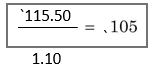
This amount is larger than what the investor has been asked to give up today. She would, therefore, accept the offer. This simple example illustrates two most common methods of adjusting cash flows for time value of money: compounding—the process of calculating future values of cash flows and discounting—the process of calculating present values of cash flows.
We just developed logic for deciding between cash flows that are separated by a period, such as one year. But most investment decisions involve more than one period. To solve such multi-period investment decisions, we simply need to extend the logic developed above. Let us assume that an investor requires 10 per cent interest rate to make him indifferent to cash flows one year apart. The question is: how should he arrive at comparative values of cash flows that are separated by two, three or any number of years?
Once the investor has determined his interest rate, say, 10 per cent, he would like to receive at least `1.10 after one year or 110 per cent of the original investment of `1 today. A two-year period is two successive one-year periods. When the investor invested `1 for one year, he must have received `1.10 back at the end of that year in exchange for the original `1. If the total amount so received (`1.10) were reinvested, the investor would expect 110 per cent of that amount, or `1.21 = `1 × 1.10 × 1.10 at the end of the second year. Notice that for any time after the first year, he will insist on receiving interest on the first year’s interest as well as interest on the original amount (principal). Compound interest is the interest that is received on the original amount (principal) as well as on any interest earned but not withdrawn during earlier periods. Compounding is the process of finding the future values of cash flows by applying the concept of compound interest. Simple interest is the interest that is calculated only on the original amount (principal), and thus, no compounding of interest takes place.
Future Value of a Single Cash Flow
Suppose your father gave you `100 on your eighteenth birthday. You deposited this amount in a bank at 10 per cent rate of interest for one year. How much future sum would you receive after one year? You would receive `110: Furture sum = Principal + Interest
= 100 + (0.10 × 100) = 100 × (1.10) = `110
What would be the future sum if you deposited `100 for two years? You would now receive interest on interest earned after one year:
Future sum = [100 + 0.10 × 100) + 0.10[100 + (0.10 × 100)]
= 100 × 1.10 × 1.10 = `121
You could similarly calculate future sum for any number of years. We can express this procedure of calculating compound, or future, value in formal terms.
Let i represent the interest rate per period, n the number of periods before pay-off, and F the future value, or compound value. If the present amount P is invested at i rate of interest for one year, then the future value F1 (viz., principal plus interest) at the end of one year will be
F1 = P + P × i = P(1 + )i
The outstanding amount at the beginning of second year is: F1 = P (1 + i). The compound sum at the end of second year will be:
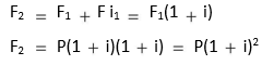
Similarly, F3 = F2(1 + i) = P(1 + i)3, and so on. The general form of equation for calculating the future value of a lump sum after n periods may, therefore, be written as follows:
Fn = P (1 + i)n (2)
The term (1+ i)n is the compound value factor (CVF) of a lump sum of `1, and it always has a value greater than 1 for positive i, indicating that CVF increases as i and n increase.
The compound value can be computed for any lump sum amount at i rate of interest for n number of years, using the given equation.
ILLUSTRATION 3.1: Future Value of a Lump Sum
Suppose that `1,000 are placed in the savings account of a bank at 5 per cent interest rate. How much shall it grow at the end of three years? It will grow as follows:
F1 = 1,000.00 + 1,000.00 × 5%
= 1,000.00 + 50.00 = `1,050.00 F2 = 1,050.00 + 1,050.00 × 5%
= 1,050.00 + 52.50 = `1,102.50 F3 = 1,102.50 + 1,102.50 × 5%
= 1,102.50 + 55.10 = `1,157.60
`55.10 on `1,102.50. In compounding, interest on interest is earned. Thus the compound value of `1,000 in the example can also be calculated as follows:
Notice that the amount of `1,000 will earn interest of `50 and will grow to `1,050 at the end of the first year. The outstanding balance of `1,050 in the beginning of the second year will earn interest of `52.50, thus making the outstanding amount equal to `1,102.50 at the beginning of the third year. Future or compound value at the end of third year will grow to `1,157.60 after earning interest of
F1 1,000 × 1.05 `1,050
F2 1,000 × [1.05 × 1.05] 1,000 × 1.052
1,000 × 1.1025 `1,102.50
F3 1,000 × [1.05 × 1.05 × 1.05] 1,000 × 1.053
1,000 × 1.1576 `1,157.60
We can see that the compound value factor (CVF) for a lump sum of one rupee at 5 per cent, for one year is 1.05, for two years 1.1025 and for three years 1.1576.
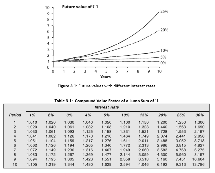
In Figure 3.1, we show the future values of `1 for different interest rates. You can see from the figure that as the interest rate increases, the compound value of `1 increases appreciably.
(2) With the help of a scientific calculator, the simple method of calculating future value is to use the power function. Suppose you have to calculate future value of `1,000 for 5 years, at 10 per cent rate of interest. In the calculator, you enter, 1.10, press the yx key, press 5 and then the equal to key =. You shall obtain 1.611. This is the CVF of `1 at 10 per cent for 5 years. Multiplying this factor by `1,000, you get the future value of `1,000 as `1,000 × 1.611 = `1,611. However, without a calculator, calculations of compound value will become very difficult if the amount is invested for a very long period. A table of future values, such as Table 3.1, can be used. Table A, given at the end of this book, is a more comprehensive table of future values.
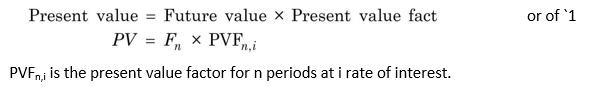
To compute the future value of a lump sum amount, we should simply multiply the amount by compound value factor (CVF) for the given interest rate, i and the time period, n from Table A. Equation (2) can be rewritten as follows:
Fn is the future or compound value after n number of periods, and CVFn,i the compound value factor for n periods at i rate of interest. As stated earlier, the compound value factor is always greater than 1.0 for positive interest rates, indicating that present value will always grow to a larger compound value.
ILLUSTRATION 3.2: Future Value of Bank Deposit
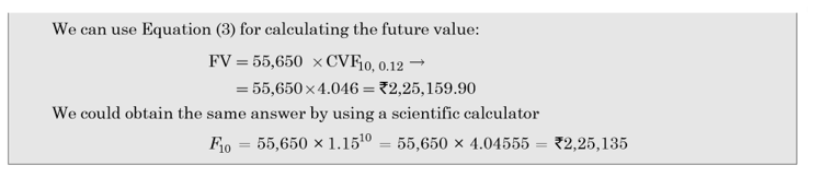
If you deposited `55,650 in a bank, which was paying a 15 per cent rate of interest on a ten-year time deposit, how much would the deposit grow at the end of ten years?
We will first find out the compound value factor at 15 per cent for 10 years. Referring to Table 3.1 (or Table A at the end of the book) and reading tenth row for 10-year period and 15 per cent column, we get CVF of `1 as 4.046. Multiplying 4.046 by `55,650, we get `2,25,159.90 as the compound value.
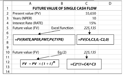
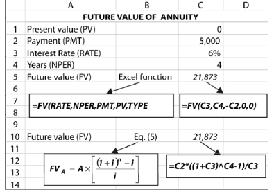
We can use the Excel’s built-in function, FV, to find out the future value of a single cash flow. FV function is given as follows:
FV (RATE, NPER, PMT, PV, TYPE)
RATE is the discount or the interest rate for a period. NPER is the number of periods. PV is the present value. PMT is the equal payment (annuity) each period and TYPE indicates the timing of cash flow, occurring either in the beginning or at the end of the period. PMT and TYPE parameters are used while dealing with annuities. In the calculation of the future value of a single cash flow, we will set them to 0.
| We can use the Excel’s built-in function, FV, to find out the future value of a single cash flow. FV function is given as follows:
FV (RATE, NPER, PMT, PV, TYPE) RATE is the discount or the interest rate for a period. NPER is the number of periods. PV is the present value. PMT is the equal payment (annuity) each period and TYPE indicates the timing of cash flow, occurring either in the beginning or at the end of the period. PMT and TYPE parameters are used while dealing with annuities. In the calculation of the future value of a single cash flow, we will set them to 0. In the worksheet above, we use the values of parameters as given in Illustration 3.2. You can find the future value in C5 by entering the formula: FV (C4, C3, 0, –C2, 0). We get the same result as in Illustration 3.2. We enter negative sign for PV; that is –C2. If we do not do so, we shall obtain negative value for FV. You can also find the future value if you write the formula for Equation (2) as given in column C10. |
FUTURE VALUE OF AN ANNUITY
Annuity is a fixed payment (or receipt) each year for a specified number of years. If you rent a flat and promise to make a series of payments over an agreed period, you have created an annuity. The equal-instalment loans from the house financing companies or employers are common examples of annuities. The compound value of an annuity cannot be computed directly from Equation (2). Let us illustrate the computation of the compound value of an annuity.
Suppose a constant sum of `1 is deposited in a savings account at the end of each year for four years at 6 per cent interest. This implies that `1 deposited at the end of the first year
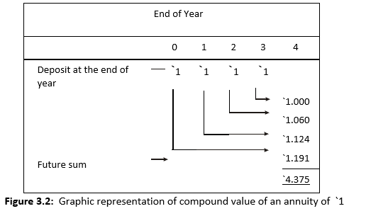
will grow for 3 years, `1 at the end of second year for 2 years, `1 at the end of the third year for 1 year and `1 at the end of the fourth year will not yield any interest. Using the concept of the compound value of a lump sum, we can compute the value of annuity. The compound value of `1 deposited in the first year will be: 1 × 1.063 = `1.191, that of `1 deposited in the second year will be: `1 × 1.062 = `1.124 and `1 deposited at the end of third year will grow to: `1 × 1.061= `1.06 and `1 deposited at the end of fourth year will remain `1. The aggregate compound value of `1 deposited at the end of each year for four years would be: 1.191 + 1.124 + 1.060 + 1.00 = `4.375. This is the compound value of an annuity of `1 for four years at 6 per cent rate of interest. The graphic presentation of the compound value of an annuity of `1 is shown in Figure 3.2. It can be seen that for a given interest rate, the compound value increases over a period.
The computations shown in Figure 3.2 can be expressed as follows:
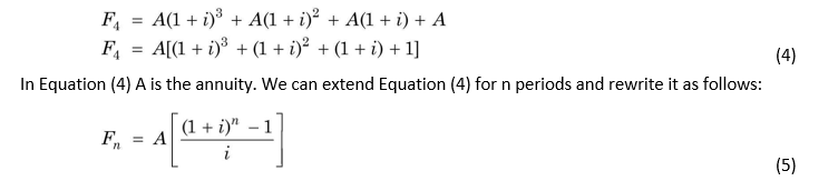
The term within brackets is the compound value factor for an annuity of `1, which we shall refer as CVFA. Consider an example.
ILLUSTRATION 3.3: Future Value of an Annuity
Suppose a firm deposits `5,000 at the end of each year for four years at 6 per cent rate of interest. How much would this annuity accumulate at the end of the fourth year? From Table B, we find that fourth year row and 6 per cent column give us a CVFA of 4.3746. If we multiply 4.375 by `5,000, we obtain a compound value of `21,875:
F4 5,000(CVFA 4,0.06 ) 5,000 × 4.3746 `21,873
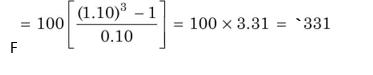
Suppose `100 are deposited at the end of each of the next three years at 10 per cent interest rate. With a scientific calculator, the compound value, using Equation (5) is calculated as follows:
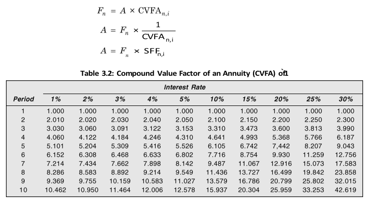
It would be quite difficult to solve Equation (5) manually if n is very large. Either using a scientific calculator or a table, (like Table 3.2), of pre-calculated compound values of an annuity of `1 can facilitate our calculations. Table B at the end of this book gives compound value factors for an annuity of `1 for a large combinations of time periods (n) and rates of interest (i). Table B is constructed under the assumption that the funds are deposited at the end of a period. CVFA should be ascertained from the table to find out the future value of the annuity. We can also write Equation (5) as follows:
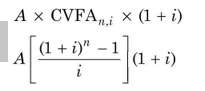
Future value = Annuity cash flow × Compound value factor for annuity of `1
Fn = A × CVFAn, i (6)
CVFAn,i is the compound value factor of an annuity of `1 for n number of years at i rate of interest.
The Excel FV function for annuity is the same as for a single cash flow. Here we are given the value for PMT instead of PV. We will set a value with negative sign for PMT (annuity) and a zero value for PV. We use the values for the parameters as given in Illustration 3.3. In column C5 we write the formula: FV (C3, C4, -C2, 0, 0). FV of `21,873 is the same as in Illustration 3.3.
Instead of the built-in Excel function, we can directly use Equation (5) to find the future value. We will get the same result. You can enter the formula in column C10 and verify the result.
Sinking Fund
Suppose we want to accumulate `21,875 at the end of four years from now. How much should we deposit each year at an interest rate of 6 per cent so that it grows to `21,875 at the end of fourth year? We know from Il lustration 3.3 that the answer is `5,000 each year. The problem posed is the reversal of the situation in Illustration 3.3; we are given the future amount and we have to calculate the annual payments. Sinking fund is a fund, which is created out of fixed payments each period to accumulate to a future sum after a specified period. For example, companies generally create sinking funds to retire bonds (debentures) on maturity.
The factor used to calculate the annuity for a given future sum is called the sinking fund factor (SFF). It is equal to the reciprocal of the compound value factor for an annuity. In Illustration 3.3, the reciprocal of CVFA of 4.3746 is: 1/4.3746 = 0.2286. When we multiply the future sum of `21,875 by SFF of 0.2286, we obtain an annuity of `5,000. The problem can be written as follows:
The Excel function for finding an annuity for a given future amount is as follows:
PMT (RATE, NPER, PV, FV, TYPE)
We use the values for the parameters as given in Illustration 3.3. In column C5 we write the formula: FV (C5, C4, –C2, –C3, 0). Note that we input both FV and PV and enter negative sign for PMT. The value of PMT is `5,000.
Instead of the built-in Excel function, we can enter formula or Equation (7) and find the value of the sinking fund (annuity). We will get the same result. You can enter the formula in column C11 and verify the result.
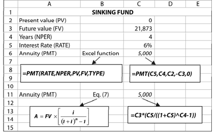
The formula for sinking fund can be written as follows as well:
Future value
Sinking fund (annuity) =
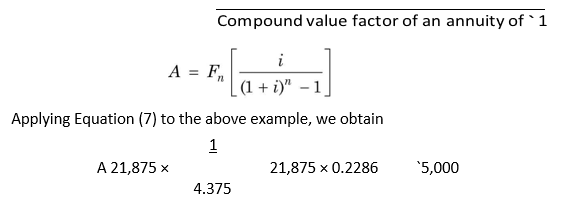
The sinking fund factor is useful in determining the annual amount to be put in a fund to repay bonds or debentures at the end of a specified period.
Check Your Concepts
- What do you understand by compounding?
- How do you compute future value of a lump sum amount and an annuity?
- What is a sinking fund? How is it calculated?
PRESENT VALUE
ILLUSTRATION 3.4: Present Value of a Lump Sum
We have so far shown how compounding technique can be used for adjusting for the time value of money. It increases an investor’s analytical power to compare cash flows that are separated by more than one period, given the interest rate per period. With the compounding technique, the amount of present cash can be converted into an amount of cash of equivalent value in future. However, it is a common practice to translate future cash flows into their present values. Present value of a future cash flow (inflow or outflow) is the amount of current cash that is of equivalent value to the decision maker. Discounting is the process of determining present values of a series of future cash flows. The compound interest rate used for discounting cash flows is also called the discount rate.
Suppose an investor wants to find out the present value of `50,000 to be received after 15 years. The interest rate is 9 per cent. First, we will find out the present value factor from Table C. When we read row 15 and 9 per cent column, we get 0.275 as the present value factor. Multiplying 0.275 by `50,000, we obtain `13,750 as the present value:
PV 50,000 × PVF15,0.09 50,000 × 0.275 `13,750
What would be the present value if `50,000 were received after 20 years? The present value factor (PVF) for 20 years at 9 per cent rate of interest is 0.178. Thus the present value of `50,000 is 50,000 × 0.178 = `8,900.
Present Value of a Single Cash Flow
We have shown earlier that an investor with an interest rate i, of say, 10 per cent per year, would remain indifferent between `1 now and `1 × 1.101 = `1.10 one year from now, or `1 × 1.102 = `1.21 after two years, or `1 × 1.103 = `1.33 after 3 years. We can say that, given 10 per cent interest rate, the present value of `1.10 after one year is: 1.10/1.101 = `1; of `1.21 after
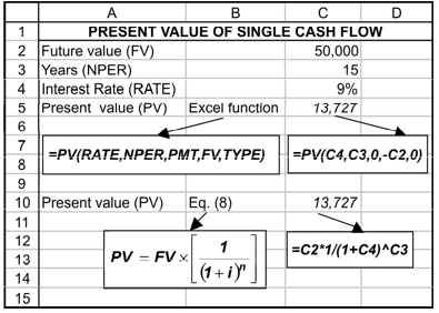
| EXCEL APPLICATION 3.4: Present Value of a Single Cash Flow |
We can find the present value of a single cash flow in Excel by using the built-in PV function:
PV (RATE, NPER, PTM, FV, TYPE)
The function is similar to FV function except the change in places for PV and FV.
We use the values of parameters as given in Illustration. We enter in column C5 the formula: PV (C4, C3, 0, –C2, 0). We get the same result as in Illustration 3.4. We enter negative sign for FV; that is –C2. This is done to avoid getting the negative value for PV.
You can also find the present value by directly using Equation (8). You write the formula for Equation (8) as given in column C10 and obtain exactly the same results.
two years is: 1.21/1.102 = `1; of `1.331 after three years is: 1.331/1.103 = `1. We can now ask a related question: How much would the investor give up now to get an amount of `1 at the end of one year? Assuming a 10 per cent interest rate, we know that an amount sacrificed in the beginning of year will grow to 110 per cent or 1.10 after a year. Thus the amount to be sacrificed today would be: 1/1.10 = `0.909. In other words, at a 10 per cent rate, `1 to be received after a year is 110 per cent of `0.909 sacrificed now. Stated differently, `0.909 deposited now at 10 per cent rate of interest will grow to `1 after one year. If `1 is received after two years, then the amount needed to be sacrificed today would be: 1/1.102 = `0.826.
How can we express the present value calculations formally? Let i represent the interest rate per period, n the number of periods, F the future value (or cash flow) and P the present value (cash flow). We know the future value after one year, F1 (viz., present value (principal) plus interest), will be:
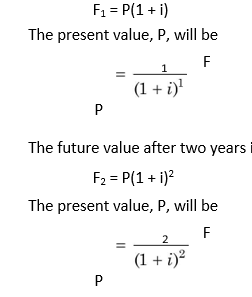
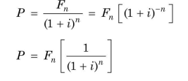
The present values can be worked out for any combination number of years and interest rate. The following general formula can be employed to calculate the present value of a lump sum to be received after some future periods:
The term in parentheses is the discount factor or present value factor (PVF), and it is always less than 1.0 for positive i, indicating that a future amount has a smaller present value. We can rewrite Equation (8) as follows:
When we want to calculate the present value factor, we can use a scientific calculator. Alternatively, we can use a table of pre-calculated present value factors like Table 3.3. You can refer to Table C at the end of this book, which gives the pre-calculated present values of `1 after n number of years at i rates of interest. To find out the present value of a future amount, we have simply to find out the present value factor (PVF) for given n and i from Table C and multiply by the future amount.
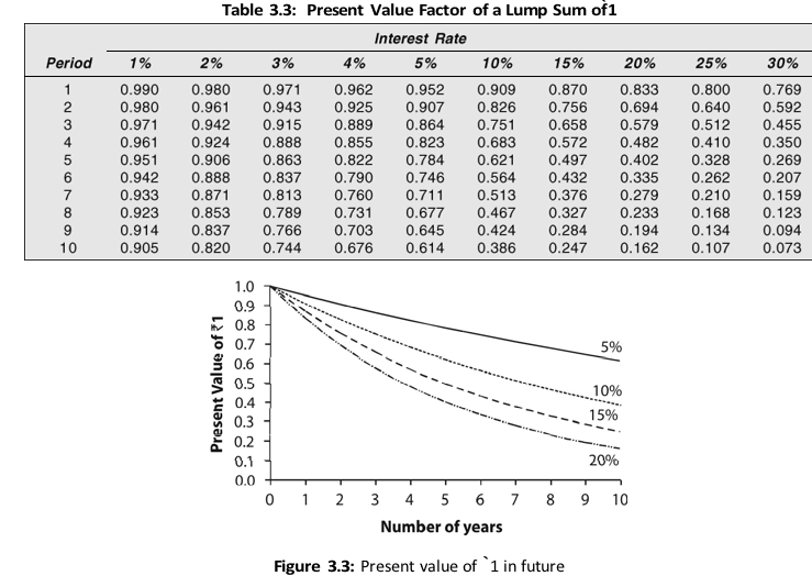
The present values decline for given interest rate as the time period increases. Similarly, given the time period, present values would decline as the interest rate increases. In Figure 3.3, we show the present value of `1 (Y-axis) for different rates over a period of time. It can be seen from the figure that the present value declines as interest rates increase and the time lengthens.
Present Value of an Annuity
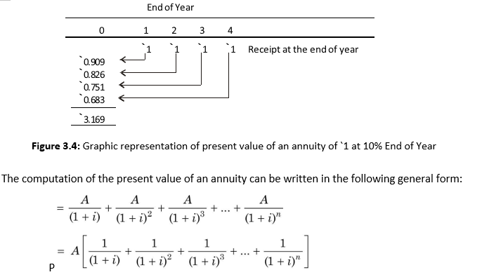
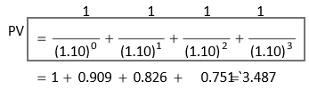
An investor may have an investment opportunity of receiving an annuity—a constant periodic amount—for a certain specified number of years. The present value of an annuity cannot be found out by using Equation (8). We will have to find out the present value of the annual amount every year and will have to aggregate all the present values to get the total present value of the annuity. For example, an investor, who has a required interest rate as 10 per cent per year, may have an opportunity to receive an annuity of `1 for four years. The present value of `1 received after one year is, P = 1/(1.10) = `0.909, after two years, P = 1/(1.10)2 = `0.826, after three years, P = 1/(1.10)3 = `0.751 and after four years, P = 1/(1.10)4 = `0.683. Thus the total present value of an annuity of `1 for four years is `3.169 as shown below:
If `1 were received as a lump sum at the end of the fourth year, the present value would be only `0.683. Notice that the present value factors of `1 after one, two, three and four years can be separately ascertained from Table C, given at the end of this book, and when they are aggregated, we obtain the present value of the annuity of `1 for four years. The present value of an annuity of `1 for four years at 10 per cent interest rate is shown in Figure 3.4. It can be noticed that the present value declines over period for a given discount rate.
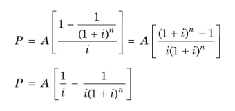
A is a constant cash flow each year. The above equation can be solved and expressed in the following alternate ways:
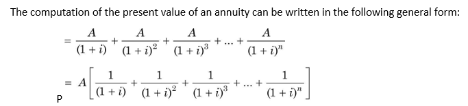
The term within parentheses of Equation (10) is the present value factor of an annuity of `1, which we would call PVFA, and it is a sum of single-payment present value factors.
To illustrate, let us suppose that a person receives an annuity of `5,000 for four years. If the rate of interest is 10 per cent, the present value of `5,000 annuity is:
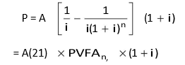
Present value = Annuity × Present value of an annuity factor of `1
It can be realised that the present value calculations of an annuity for a long period would be extremely cumbersome without a scientific calculator. We can use a table of the pre-calculated present values of an annuity of `1 as shown in Table 3.4. Table D at the end of this book gives present values of an annuity of `1 for numerous combinations of time periods and rates of interest. To compute the present value of an annuity, we should simply find out the appropriate factor from Table D and multiply it by the annuity value. In our example, the value 3.170, solved by using Equation (10), could be ascertained directly from Table D. Reading fourth year row and 10 per cent column, the value is 3.170. Equation (10) can also be written as follows:
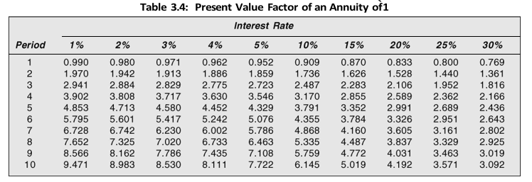
PVFAn,i is present value factor of an annuity of `1 for n periods at i rate of interest. Applying the formula and using Table D, we get:
PV = 5,000 (PVFA4,0.10) = 5,000 × 3.170 = `15,850
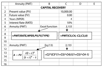
The Excel function for finding an annuity (capital recovery) for a given present value is the same as for finding the sinking fund. PV replaces FV in the formula.
We use the values for the parameters as given in the example above. In column C5 we write the formula: FV (C5, C4, –C2, C3, 0). Note that we input both FV and PV and enter negative sign for PMT. The value of PMT is `3,155.
Instead of the built-in Excel function, we can enter the formula for Equation (13) and find the value of the capital recovery (annuity). We will get the same result. You can enter the formula for Equation (13) in column C11 and verify the result.
Present Value of Perpetuity
Perpetuity is an annuity that occurs indefinitely. Perpetuities are not very common in financial decision-making. But one can find a few examples. For instance, in the case of irredeemable preference shares (i.e., preference shares without a maturity), the company is expected to pay preference dividend perpetually. By definition, in a perpetuity, time period, n, is so large (mathematically n approaches infinity, ) that the expression (1 + i)n in Equation (10) tends to become zero, and the formula for a perpetuity simply becomes
Perpetuity
Present value of a perpetuity =
Interest rate

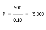
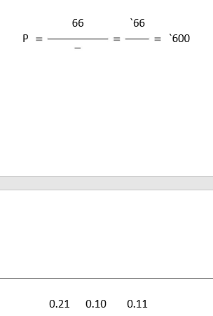
To take an example, let us assume that an investor expects a perpetual sum of `500 annually from his investment. What is the present value of this perpetuity if interest rate is 10 per cent? Applying Equation (14), we get:
Present Value of an Uneven Cash Flow
Investments made by a firm do not frequently yield constant periodic cash flows (annuity). In most instances the firm receives a stream of uneven cash flows. Thus the present value factors for an annuity, as given in Table D (at the end of the book), cannot be used. The procedure is to calculate the present value of each cash flow (using Table C) and aggregate all present values. Consider the illustration 3.6.
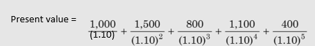
ILLUSTRATION 3.6: Present Value of Uneven Cash Flows
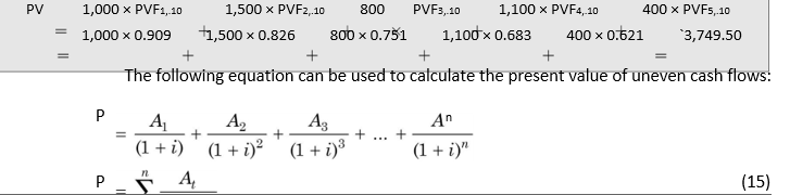
Consider that an investor has an opportunity of receiving `1,000, `1,500, `800, `1,100 and `400, respectively, at the end of one through five years. Find out the present value of this stream of uneven cash flows, if the investor’s required interest rate is 10 per cent. The present value is calculated as follows:
The complication of solving this equation can be resolved by using Table B at the end of the book. We can find out the appropriate present value factors (PVFs) either from Table B (at the end of the book) or by using a calculator and multiply them by the respective amount. The present value calculation is shown below:
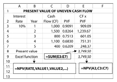
We can set the Excel worksheet to find the present value of an uneven series of cash flows. In the worksheet below, the values for cash flows are entered in column C3 to column C7. Years are entered in column B3 to column B7 and interest rate (10%) in column A3. In column D3 to D7 we have entered formula for the present value factor (PVF) for a single cash flow. For example, you can enter in column D3 the formula: [(1/(1+$A$3)^B3…Bn] for all columns and copy it to other columns, while changing B3 to B4 … B7 respectively. Since the interest rate will be same for all years, we have set it constant by entering $A$3. When you multiply the values in column C by the values in column D, you obtain the present value of each cash flow in column E. The total present value is the sum of all individual present values. You can get the total present value in column E8 by entering the formula: = SUM (E3:E7).
You can also use the built-in Excel function NPV to calculate the present value of uneven cash flows:
NPV(RATE,VALUE1,VALUE2,…)
We enter in column E9 the formula: NPV (A3, C3:C7). We get the same result as above. Note that there is no cash flow in year 0.
In Equation (15) t indicates number of years, extending from one year to n years. In operational terms, Equation (15) can be written as follows
![]()
Present Value of Growing Annuity
In financial decision-making there are number of situations where cash flows may grow at a constant rate. For example, in the case of companies, dividends are expected to grow at a constant rate. Assume that to finance your post-graduate studies in an evening college, you undertake a part-time job for 5 years. Your employer fixes an annual salary of `1,000 with the provision that you will get annual increment at the rate of 10 per cent. It means that you shall get the following amounts from year 1 through year 5.

If your required rate of return is 12 per cent, you can use the following formula to calculate the present value of your salary:
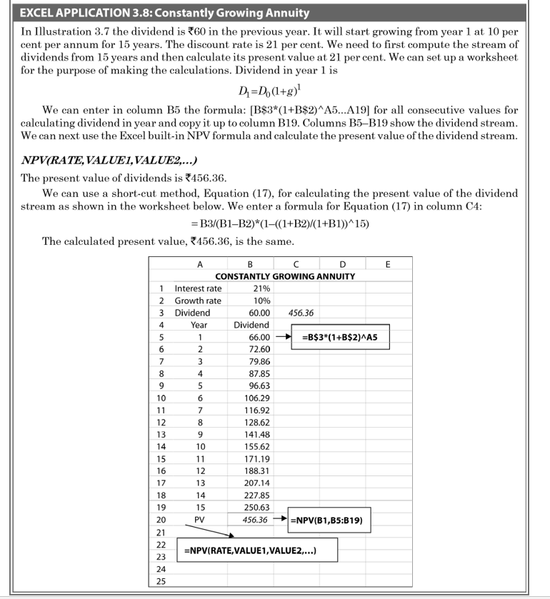
The problem in Illustration 3.7 is quite involved. You can easily solve it with a scientific calculator. Alternatively, you can use Excel spreadsheet to solve it (as shown in Excel application 3.8).
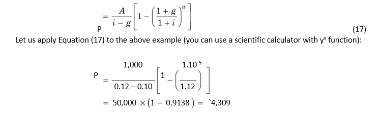
ILLUSTRATION 3.7: Value of a Growing Annuity
A company paid a dividend of `60 last year. The dividend stream commencing from year one is expected to grow at 10 per cent per annum for 15 years and then end. If the discount rate is 21 per cent, what is the present value of the expected series?
There is a long way to solve this problem. You may first calculate the series of dividends over 15 years. Note that the first annuity (dividend) in year 1 will be: 60 × 1.10 = `66. Similarly, dividends for other years can be calculated. Once the dividends have been worked out, you can find their present value using the 21 per cent discount rate. This
procedure is shown under Excel Application 3.8. You can use Equation (17) to find the present value of the series of dividend as follows:
A 1 g n
P 1
i g 1 i
15
66 1.10
P 1
0.21 0.10 1.21
600 (1 0.90915 ) 600 0.7606 `456.36
Present Value of Growing Perpetuities
Constantly growing perpetuities are annuities growing indefinitely. How can we value a constantly growing perpetuity? Suppose dividends of `66 after year one in Illustration 3.7 are expected to grow at 10 per cent indefinitely. The discount rate is 21 per cent. Hence, the present value of dividends will be as follows:
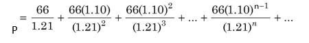
In mathematical term, we may say that in Equation (17), n—the symbol for the number of years—is not finite and that it extends to infinity ( ). Then the calculation of the present value of a constantly growing perpetuity is given by a simple formula as follows:
Thus, in Illustration 3.7 if the dividend of `66 in year 1 were expected to grow perpetually, the present value would be:
VALUE OF AN ANNUITY DUE
The concepts of compound value and present value of an annuity discussed earlier are based on the assumption that series of cash flows occur at the end of the period. In practice, cash flows could take place at the beginning of the period. When you buy a fridge on an instalment basis, the dealer requires you to make the first payment immediately (viz., in the beginning of the first period) and subsequent instalments in the beginning of each period. It is common in lease or hire purchase contracts that lease or hire purchase payments are required to be made in the beginning of each period. Lease is a contract to pay lease rentals (payments) for the use of an asset. Hire purchase contract involves regular payments (instalments) for acquiring (owning) an asset. Annuity due is a series of fixed receipts or payments starting at the beginning of each period for a specified number of periods.
Future Value of an Annuity Due
How can we compute the compound value of an annuity due? Suppose you deposit `1 in a savings account at the beginning of each year for 4 years to earn 6 per cent interest? How much will be the compound value at the end of 4 years? You may recall that when deposit of `1 made at the end of each year, the compound value at the end of 4 years is `4.375 (see Figure 3.2). However, `1 deposited in the beginning of each of year 1 through year 4 will earn interest, respectively, for 4 years, 3 years, 2 years and 1 year:
F 1 × 1.064 1 × 1.063 1 × 1.062 1 × 1.061
1.262 1.191 1.124 1.06 `4.637
You can see that the compound value of an annuity due is more than of an annuity because it earns extra interest for one year. If you multiply the compound value of an annuity by (1+ i), you would get the compound value of an annuity due. The formula for the compound value of an annuity due is as follows:
Future value of an annuity due = Future value of an annuity × (1 + i) = (19)
Thus the compound value of `1 deposited at the beginning of each year for 4 years is
1 × 4.375 × 1.06 = `4.637
The compound value annuity factors in Table B (at the end of the book) should be multiplied by (1 + i) to obtain relevant factors for an annuity due.
Present Value of an Annuity Due
Let us consider a 4-year annuity of `1 each year, the interest rate being 10 per cent. What is the present value of this annuity if each payment is made at the beginning of the year? You may recall that when payments of `1 are made at the end of each year, then the present value of the annuity is `3.169 (see Figure 3.4). Note that if the first payment is made immediately, then its present value would be the same (i.e., `1) and each year’s cash payment will be discounted by one year less. This implies that the present value of an annuity due would be higher than the present value of an annuity. Thus, the present value of the series of `1 payments starting at the beginning of a period is
The formula for the present value of an annuity due is:
Present value of an annuity due = Present value of an annuity × (1 + i)
You can see that the present value of an annuity due is more than of an annuity by the factor of (1 + i). If you multiply the present value of an annuity by (1 + i), you would get the present value of an annuity due.
Applying Equation (21), the present value of `1 paid at the beginning of each year for
4 years is
1 × 3.170 × 1.10 = `3.487
MULTI-PERIOD COMPOUNDING
The present value annuity factors in Table D (at the end of the book) should be multiplied by (1 + i) to obtain relevant factors for an annuity due.
We have assumed in the discussion so far that cash flows occurred once a year. In practice, cash flows could occur more than once a year. For example, banks may pay interest on savings account quarterly. On bonds or debentures and public deposits, companies may pay interest semi-annually. Similarly, financial institutions may require corporate borrowers to pay interest quarterly or half-yearly.
The interest rate is usually specified on an annual basis, in a loan agreement or security (such as bonds), and is known as the nominal interest rate. If compounding is done more than once a year, the actual annualized rate of interest would be higher than the nominal interest rate and it is called the effective interest rate. Consider an example.
Suppose you invest `100 now in a bank, interest rate being 10 per cent a year, and that the bank will compound interest semi-annually (i.e., twice a year). How much amount will you get after a year? The bank will calculate interest on your deposit of `100 for first six months at 10 per cent and add this interest to your principal. On this total amount accumulated at the end of first six months, you will again receive interest for next six months at 10 per cent. Thus, the amount of interest for first six months will be:
Interest = `100 × 10% × ½ = `5
and the outstanding amount at the beginning of the second six-month period will be: `100 + `5 = `105. Now you will earn interest on `105. The interest on `105 for next six months will be:
Interest = `105 × 10% × ½ = `5.25
Thus you will accumulate `100 + `5 + `5.25 = `110.25 at the end of a year. If the interest were compounded annually, you would have received: `100 + 10% × `100 = `110. You received more under semi-annual compounding because you earned interest on interest earned during the first six months. You will get still higher amount if the compounding is done quarterly or monthly.
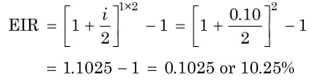
What effective annual interest rate did you earn on your deposit of `100? On an annual basis, you earned `10.25 on your deposit of `100; so the effective interest rate (EIR) is:
This implies that `100 compounded annually at 10.25 per cent, or `100 compounded semi-annually at 10 per cent will accumulate to the same amount.
EIR in the above example can also be found out using Equation( 22):
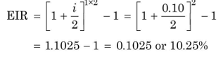
Notice that annual interest rate, i, has been divided by 2 to find our semi-annual interest rate since we want to compound interest twice, and since there are two compounding periods in one year, the term (1 + i/ 2) has been squared. If the compounding is done quarterly, the annual interest rate, i, will be divided by four and there will be four compounding periods in one year. This logic can be extended further as shown in Illustration 3.8.
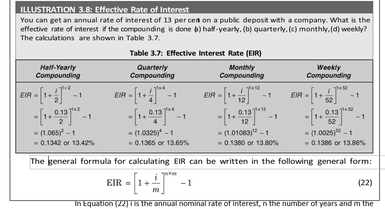
number of compounding per year. In annual compounding, m = 1, in monthly compounding m = 12 and in weekly compounding m = 52.
The concept developed in Equation 22 can be used to accomplish the multi-period compounding or discounting for any number of years. For example, if a company pays 15 per cent interest, compounded quarterly, on a 3-year public deposit of `1,000, then the total amount compounded after 3 years will be:
We can thus use the Equation (22) for computing the compounded value of a sum in case of the multi-period compounding:
The logic developed above can be extended to compute the present value of a sum or an annuity in case of the multi-period compounding. The discount rate will be i/m and the time horizon will be equal to n × m.
We can set up a worksheet as shown below to see the effect of the multi-period compounding. In column C we calculate the future value of `1 at 12 per cent annual rate for different compounding periods. In C6 we enter the formula for calculating the future value:
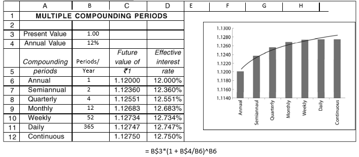
Alternatively, you can use the Excel built-in formula FV. Since the present value and interest rate are fixed, we insert the dollar sign, while changing B6 to B7, B8 … B11, respectively. For continuous compoun-ding, we enter the formula in C12 as: =B$3*exp(B$4). The built-in EXP function solves for e raised to power of a specified number. We can see that the future value increases as the frequency of compounding increases. This is also reflected through the higher effective interest rates calculated in column D. You may, however, note that the effective interest rate or future value rises slowly as the compounding frequencies increasing
Continuous Compounding
Sometimes compounding may be done continuously. For example, banks may pay interest continuously; they call it daily compounding. The continuous compounding function takes the form of the following formula:
![]()
In Equation (25), x = interest rate i multiplied by the number of years n and e is equal to 2.7183.
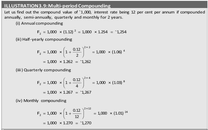
In Illustration 3.9, if the compounding is done continuously, then the compound value will be:
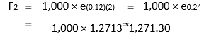
The values of ex are available in Table E at the end of the book. You can also use of scientific calculator for this purpose.
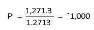
Equation (25) can be transformed into a formula for calculating present value under continuous compounding.
![]()
Thus, if `1,271.3 is due in 2 years, discount rate being 12 per cent, then the present value of this future sum is:
NET PRESENT VALUE
We have stated in Chapter 1 that the firm’s financial objective should be to maximize the shareholder’s wealth. Wealth is defined as net present value. Net present value (NPV) of a financial decision is the difference between the present value of cash inflows and the present value of cash outflows. Suppose you have `2,00,000. You want to invest this money in land, which can fetch you `2,45,000 after one year when you sell it. You should undertake this investment if the present value of the expected `2,45,000 after a year is greater than the investment outlay of `2,00,000 today. You can put your money to alternate uses. For example, you can invest `2,00,000 in units (for example, Unit Trust of India sells ‘units’ and invests money in securities of companies on behalf of investors) and earn, say, 15 per cent dividend a year. How much should you invest in units to obtain `2,45,000 after a year? In other words, if your opportunity cost of capital is 15 per cent, what is the present value of `2,45,000 if you invest in land? The present value by using Eq. 11 is:
![]()
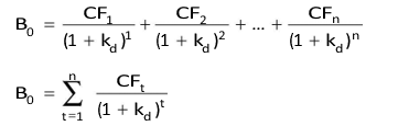
The land is worth `2,13,150 today, but that does not mean that your wealth will increase by `2,13,150. You will have to commit `2,00,000, and therefore, the net increase in your wealth or net present value is: `2,13,150 – `2,00,000 = `13,150. It is worth investing in land. The general formula for calculating NPV can be written as follows:
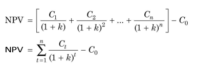
Ct is cash inflow in period t, C0 cash outflow today, k the opportunity cost of capital and t the time period. Note that the opportunity cost of capital is 15 per cent because it is the return foregone by investing in land rather than investing in securities (units), assuming risk is the same. The opportunity cost of capital is used as a discount rate.
PRESENT VALUE AND RATE OF RETURN
You may be frequently reading advertisements in newspapers: deposit, say `1,000 today and get twice the amount in 7 years; or pay us `100 a year for 10 years and we will pay you `100 a year thereafter in perpetuity. A company or financial institution may offer you bond or debenture for a current price lower than its face value and repayable in the future at the face value, but without an interest (coupon). A bond that pays some specified amount in future (without periodic interest) in exchange for the current price today is called a zerointerest bond or zero-coupon bond. In such situations, you would be interested to know what rate of interest the advertiser is offering. You can use the concept of present value to find out the rate of return or yield of these offers. Let us take some examples.
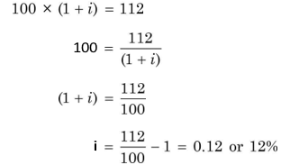
A bank offers you to deposit `100 and promises to pay `112 after one year. What rate of interest would you earn? The answer is 12 per cent:
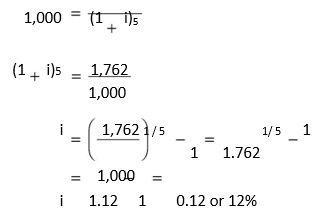
What rate of interest would you earn if you deposit `1,000 today and receive `1,762 at the end of five years? You can set your problem as follows: `1,000 is the present value of
`1,762 due to be received at the end of the fifth year. Thus,
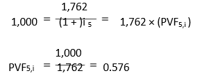
1,762
Now you refer to Table C, given at the end of the book, that contains the present value of `1. Since 0.567 is a PVF at i rate of interest for 5 years, look across the row for period 5 and interest rate column until you find this value. You will notice this factor in the 12 per cent column. You will, thus, earn 12 per cent on your `1,000. (Check: `1,000 × (1.12)5 = `1,000 × 1.762 = `1,762). You can use a scientific calculator to solve for the rate of return:
Let us take the example of an annuity. Assume you borrow `70,000 from the Housing Development Finance Corporation (HDFC) to buy a flat in Ahmedabad. You are required to mortgage the flat and pay `11,396.93 annually for a period of 15 years. What interest rate would you be paying? You may note that `70,000 is the present value of a fifteen-year annuity of `11,396.93. That is,
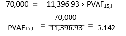
You need to look across in Table D (at the end of this book) the 15-year row and interest rate columns until you get the value 6.142. You will find this value in the 14 per cent column.
Thus HDFC is charging 14 per cent interest from you.
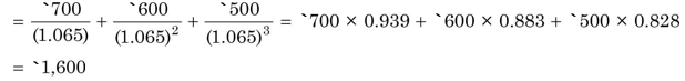
Finding the rate of return for an uneven series of cash flows is a bit difficult. By practice and using trial and error method you can find it.* Let us consider an example to illustrate the calculation of rate of return for an uneven series of cash flows.
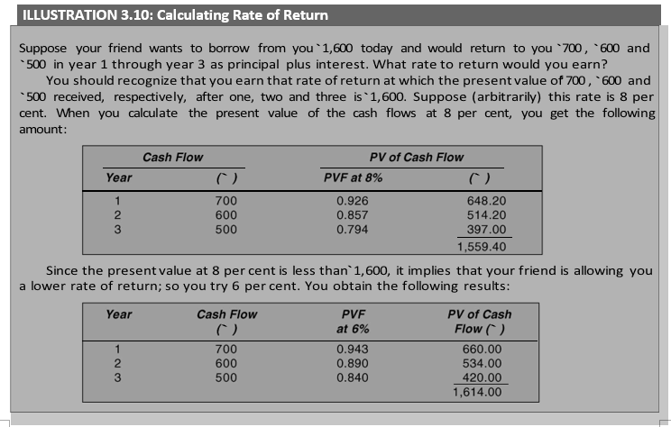
The present value at 6 per cent is slightly more than, 1,600; it means that your friend is offering you approximately 6 per cent interest. In fact, the actual rate would be a little higher than 6 per cent. At 7 per cent, the present value of cash flows is `1,586. You can interpolate as follows to calculate the actual rate:
![]()
At 6.5 per cent rate of return, present value of `700, `600 and `500 occurring respectively in year one through three is equal to `1,600:
The rate of return of an investment is called internal rate of return (IRR) or yield since it depends exclusively on the cash flows of the investment. Once you have understood the logic of the calculation of the internal rate of return, you can use a scientific calculator or Excel to find it.
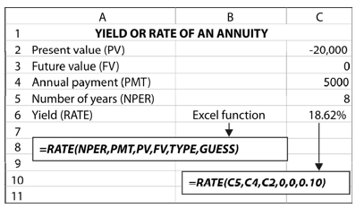
EXCEL APPLICATION 3.10: Yield or IRR Calculation
Excel has built-in functions for calculating the yield or IRR of an annuity and uneven cash flows. The Excel function to find the yield or IRR of an annuity is:
RATE(NPER,PMT,PV,FV,TYPE,GUESS)
GUESS is a first guess rate. It is optional; you can specify your formula without it. In column C6 we enter the formula: =RATE (C5, C4, C2, 0,0,0.10). The last value 0.10 is the guess rate, which you may omit to specify. For investment with an outlay of `20,000 and earning an annuity of `5,000 for 8 years, the yield is 18.62 per cent.
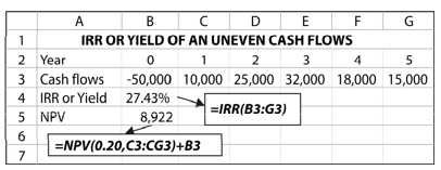
The Excel built-in function IRR calculates the yield or IRR of uneven cash flows:
IRR(VALUES,GUESS)
The values for the cash flows should be in a sequence, starting from the cash outflow. GUESS is a first guess rate (arbitrary) and it is optional. In the worksheet, we have entered the cash flows of an investment project. In column B4 we enter the formula: =IRR(B3:G3) to find yield (IRR). Note that all cash flows in year 0 to year 5 have been entered in that sequence. The yield (IRR) is 27.43 per cent.
You can also use the built-in function, NPV,
The rate of return of an investment is called internal rate of return (IRR) or yield since it depends exclusively on the cash flows of the investment. Once you have understood the logic of the calculation of the internal rate of return, you can use a scientific calculator or Excel to find it.
EXCEL APPLICATION 3.10: Yield or IRR Calculation
Excel has built-in functions for calculating the yield or IRR of an annuity and uneven cash flows. The Excel function to find the yield or IRR of an annuity is:
RATE(NPER,PMT,PV,FV,TYPE,GUESS)
GUESS is a first guess rate. It is optional; you can specify your formula without it. In column C6 we enter the formula: =RATE (C5, C4, C2, 0,0,0.10). The last value 0.10 is the guess rate, which you may omit to specify. For investment with an outlay of `20,000 and earning an annuity of `5,000 for 8 years, the yield is 18.62 per cent.
The Excel built-in function IRR calculates the yield or IRR of uneven cash flows:
IRR(VALUES,GUESS)
The values for the cash flows should be in a sequence, starting from the cash outflow. GUESS is a first guess rate (arbitrary) and it is optional. In the worksheet, we have entered the cash flows of an investment project. In column B4 we enter the formula: =IRR(B3:G3) to find yield (IRR). Note that all cash flows in year 0 to year 5 have been entered in that sequence. The yield (IRR) is 27.43 per cent.
You can also use the built-in function, NPV,
| Summary | |
| Individual investors generally prefer possession of a given amount of cash now, rather than the same amount at some future time. This time preference for money may arise because of (a) uncertainty of cash flows, (b) subjective preference for consumption, and (c) availability of investment opportunities. The last reason is the most sensible justification for the time value of money. A risk premium may be demanded, over and above the riskfree rate as compensation for time, to account for the uncertainty of cash flows. Interest rate or time preference rate gives money its value, and facilitates the comparison of cash flows occurring at different time periods. |
|
A riskpremium rate is added to the riskfree time preference rate to derive required interest rate from risky investments.
Two alternative procedures can be used to find the value of cash flows: compounding and discounting.
In compounding, future values of cash flows at a given interest rate at the end of a given period of time are found. The future value (F) of a lump sum today (P) for n periods at i rate of interest is given by the following formula:
Fn P(1 i)n P(CVFn i, )
The compound value factor, CVFn,i can be found out from Table A given at the end of the book.
The future value of an annuity (that is, the same amount of cash each year) for n periods at i rate of interest is given by the following equation.
(1 i)n 1
Fn P P(CVFAn i, )
i
The compound value of an annuity factor (CVFAn,i) can be found out from Table B given at the end of the book. The compound value of an annuity formula can be used to calculate an annuity to be deposited to a sinking fund for n periods at i rate of interest to accumulate to a given sum. The following equation can be used:
1
A F F(SFFn i, )
CVFAn i,
The sinking fund factor (SFFn,i) is a reciprocal of CVFAn,i.
In discounting, the present value of cash flows at a given interest rate at the beginning of a given period of time is computed. The present value concept is the most important concept in financial decisionmaking. The present value (P) of a lump sum (F) occurring at the end of n period at i rate of interest is given by the following equation:
Fn Fn(PVFn,i)
P 1 i)n
(
The present value factor (PVFn,i) can be obtained from Table C given at the end of the book.
The present value of an annuity (A) occurring for n periods at i rate of interest can be found out as follows:
1
1 (1 i)n (1 i)n 1 1 1
P A 1 n A i i(1 i)n A(PVFAn,i)
i i( i)
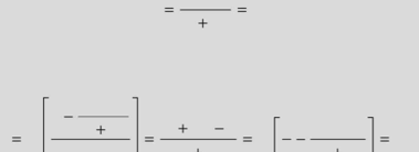
Table D at the end of this book can be used to find out the present value of annuity factor (PVFAn,i).
The present value of an annuity formula can be used to determine annual cash flows to be earned to recover a given investment. The following equation can be used:
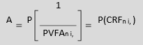
Notice that the capital recovery factor (CRFn,i) is a reciprocal of the present value annuity factor, PVFAn,i.
The present value concept can be easily extended to compute present value of an uneven series of cash flows, cash flows growing at constant rate, or perpetuity.
When interest compounds for more than once in a given period of time, it is called multiperiod compounding. If i is the nominal interest rate for a period, the effective interest rate (EIR) will be more than the nominal rate i in multiperiod compounding since interest on interest within a year will also be earned, EIR is given as follows:
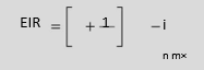
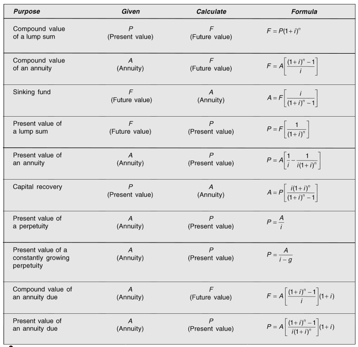
Table 3.8 gives the summary of the compounding and discounting formulae.
An important corollary of the present value is the internal rate of return (IRR). IRR is the rate which equates the present value of cash flows to the initial investment. Thus in operational terms, in the present value equation, all variables are known except i; i can be found out by trial and error method as discussed in the chapter.
Wealth or net present value of a financial decision is defined as the difference between the present value of cash inflows (benefits) and the present value of cash outflows (costs). Wealth maximisation principle uses interest rate to find out the present value of benefits and costs, and as such, it considers their timing and risk.
In view of the logic for the time value of money, the financial criterion is expressed in terms of wealth maximization. As discussed in Chapter 1, the alternate criterion of profit maximization is not only conceptually vague but it also does not take into account the timing and uncertainty of cash flows.
Review Questions
- ‘Generally individuals show a time preference for money.’ Give reasons for such a preference.
- ‘An individual’s time preference for money may be expressed as a rate.’ Explain.
- Why is the consideration of time important in financial decision making? How can time value beadjusted? Illustrate your answer.
- Is the adjustment of time relatively more important for financial decisions with short-rangeimplications or for decisions with long-range implications? Explain.
- Explain the mechanics of calculating the present value of cash flows.
- What happens to the present value of an annuity when the interest rate rises? Illustrate.
- What is multi-period compounding? How does it affect the annual rate of interest? Give an example.8. What is an annuity due? How can you calculate the present and future values of an annuity due? Illustrate.
- How does discounting and compounding help in determining the sinking fund and capital recovery?
- Illustrate the concept of the internal rate of return.