
INTRODUCTION
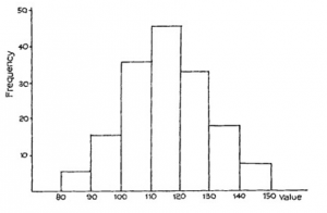
In Study Unit 4, Section E of this module, we considered various graphical ways of representing a frequency distribution. We considered a frequency dot diagram, a bar chart, a polygon and a frequency histogram. For a typical histogram, see Figure 7.1. You will immediately get the impression from this diagram that the values in the centre are much more likely to occur than those at either extreme.
Consider now a continuous variable in which you have been able to make a very large number of observations. You could compile a frequency distribution and then draw a frequency bar chart with a very large number of bars, or a histogram with a very large number of narrow groups. Your diagrams might look something like those in Figure 7.2.
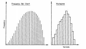
If you now imagine that these diagrams relate to relative frequency distribution and that a smooth curve is drawn through the tops of the bars or rectangles, you will arrive at the idea of a frequency curve.
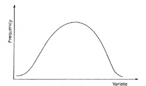
Most of the distributions which we get in practice can be thought of as approximations to distributions which we would get if we could go on and get an infinite total frequency; similarly, frequency bar charts and histograms are approximations to the frequency curves which we would get if we had a sufficiently large total frequency. In this course, from now onwards, when we wish to illustrate frequency distributions without giving actual figures, we will do so by drawing the frequency curve, as in Figure 7.3.
THE NORMAL DISTRIBUTION
The “Normal” or “Gaussian” distribution is probably the most important distribution in the whole of statistical theory. It was discovered in the early 18th century, because it seemed to represent accurately the random variation shown by natural phenomena. For example:
− heights of adult men from one race
− weights of a species of animals
− the distribution of IQ levels in children of a certain age
− weights of items packaged by a particular packing machine − life expectancy of light bulbs
A typical shape is shown in Figure 7.4. You will see that it has a central peak (i.e. it is unimodal) and that it is symmetrical about this centre.
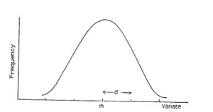
The mean of this distribution is shown as m on the diagram, and is located at the centre. The standard deviation, which is usually denoted by s, is also shown.
There are some interesting properties which these curves exhibit, which allow us to carry out calculations on them. For distributions of this approximate shape, we find that 68% of the observations are within ±1 standard deviation of the mean, and 95% are within ±2 standard deviations of the mean. For the normal distribution, these figures are exact. See Figure 7.5.
STATISTICAL INFERENCE
Introduction
Often, in real life, the mean and standard deviation of a particular population of items are not known. The population may be too large to measure them all, or it may be continuous production, and therefore impossible to measure all items. For example, consider a machine which packages a food product. These packages are marked as 500 grams and are sold by weight. The average weight of the whole population of packages is clearly important, but is unknown. The only way to arrive at an estimate is to take a sample of items from the population. Having taken a sample, you can then calculate the sample mean. Is this a good indication of the population mean? How close is it likely to be? Statistical inference is the technique of using sample statistics to estimate population statistics.
Sampling Distributions
If a sample is taken from a population, and the sample mean calculated, this can be used to estimate the population mean. Now consider what happens if a second sample is taken from the same population. Another estimate is obtained, which will probably be different from the first one. Imagine now that a large number of samples are taken, all from the same population. You can see that all the estimates obtained for the population mean can themselves be used to give a distribution. That is, the sample means have a distribution, in just the same way that the population weights have a distribution. In fact, there are very important similarities as follows:
- If the population distribution is normal, the distribution of the sample means will also be normal.
- The mean of the distribution of the sample means equals the mean of the population distribution.
The standard deviation of the distribution of sample means is smaller than the standard deviation of the population