
KEYNES AND AGGREGATE DEMAND
In the previous chapter, we were concerned with the measurement of economic activity. In this and subsequent chapters, we will be developing a system of macro-economic analysis to help us investigate why the level of economic activity is what it is. It is often the case that GDP is significantly lower than it might be. High levels of unemployment imply that economies could be producing more. What are the causes of high levels of unemployment? What conditions are necessary for economies to be operating at their full-employment level of output?
The starting point for macroeconomic analysis is usually the work of John Maynard Keynes. Keynes wished to understand why economies tended to progress in a cycle of booms and slumps (the business cycle) and why they occasionally experienced prolonged recessions. The boom periods were characterised by high and rising levels of output and employment while the slumps were characterised by rising unemployment and falling output.
Keynes put forward a simple but persuasive explanation regarding the determination of output and employment in the economy. The level of output firms will be willing to produce, he argued, is determined by the aggregate demand (AD) for goods and services in the economy. The level of output firms are willing to produce will, in turn, determine the level of employment. The level of aggregate demand drives the economy.
AD à output à employment
If total demand in the economy were to rise, firms would wish to produce more and therefore they would be offering more employment. If total demand were to fall, firms would have accumulating unsold stocks leading them to cut production and employment. If we wish to know why the levels of output and employment tend to fluctuate, according to Keynes, the explanation is to be found in fluctuations in the level of aggregate demand.
Aggregate demand is concerned with the total level of desired (or planned) expenditure in the economy and has four components originating from four different sources.
- Households: consumption expenditure (C);
- Firms: capital and inventory investment expenditure (I);
- Government: current and capital expenditure (G);
- Foreign sector: the excess of exports over imports (X – M).
AD = C + I + G + (X – M) [10.1]
Though similar to the accounting identity for GDP (see Study unit 9), aggregate demand is not the same thing as GDP. The components of aggregate demand in the above identity relate to desired levels of expenditure whereas the components in the accounting identity for GDP relate to realised outcomes. Planned and realised outcomes may not necessarily coincide, only doing so when the economy is in equilibrium.
To understand why aggregate demand might fluctuate, we need to understand why the components (C, I, G, X & M) might fluctuate. When we know this we can bring the components together to construct a theoretical model of the economy. It is important to realise that the model can take a simple form initially but be made more complex by relaxing or changing the assumptions underlying the model. The simplest model is that of a twosector closed economy. This focuses on the interaction between domestic households and firms while ignoring the impact of government and the foreign sector. By adding a government to the model we have a closed economy with government. By adding the foreign sector we move to an open economy model. While simple models can be accused of lacking realism, they are essential for developing the analysis by enabling us to isolate and focus on key macroeconomic relationships.
TWO SECTOR MODEL
Consumption and Savings Functions
It is convenient to think of households and firms as being completely distinct. Households derive their incomes (wages, rent, interest, profit) from the factor services they provide to firms. If we assume that all the profit earned by firms is distributed then gross factor incomes is equal to GDP.
Households have a simple choice with regard to the income they receive; they can either spend it or save it. If total income is denoted with a Y, total household spending with a C and total household savings with an S, we have:
Y = C + S [10.2]
The consumption function is concerned with all factors that may influence the level of consumption expenditure. The savings function is concerned with all factors that influence the level of savings. The single most important influence on the level of household consumption expenditure (C) is the level of household income (Y). It is assumed that as Y rises C will also rise, but not by the same amount. As Y rises, household savings (S) will also rise, therefore;
∆Y = ∆C + ∆S [10.3]
where ∆C and ∆S are both positively related to ∆Y.
The proportion of any change in income that is spent is known as the marginal propensity to consume (MPC) while the proportion that is saved is known as the marginal propensity to save (MPS).
Example:
Household income rises by RWF100m and as a result consumption expenditure rises by RWF80m and savings rise by RWF20m.
MPC = ∆C = 80 = 0.8
∆Y 100
MPS = ∆S = 20 = 0.2 ∆Y 100
It also follows that:
MPC + MPS = 1 [10.4]
The proportion of any given level of income that is spent is known as the average propensity to consume (APC) while the proportion that is saved is known as the average propensity to save (also known as the savings ratio):
APC + APS = C+S = 1 [10.5] Y Y
The general shape of the consumption function and the savings function are as illustrated in Figure 10.1. The diagrams indicate that both consumption expenditure and savings rise as income rises. The slope of the savings function at any point is the MPS. By assumption the slopes are positive but less than one. The APC at any point on the consumption function is simply the level of consumption over the corresponding level of income (e.g. APC at point a is c0/y0). The APS at any point on the savings function is the level of savings over the corresponding level of income (e.g. APC at point b is s0/y0).
Other factors that are likely to influence the level of income spent or saved include:
- the market rate of interest (i);
- household wealth.
Rising interest rates will make saving more attractive and, by implication, consumption expenditure less attractive. If interest rates rise, the proportion of income spent (APC) will fall while the proportion saved (APS) will rise and vice versa.
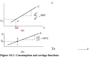
Figure 10.1: Consumption and savings functions
Increases in household wealth, e.g. an increase in the value of the housing stock, will mean that households will be less likely to save and more likely to spend and vice versa. Any changes, other than changes in household income, that cause C or S to change can be illustrated by a shift in the consumption and savings functions.
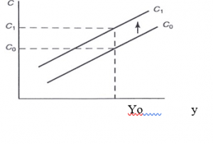
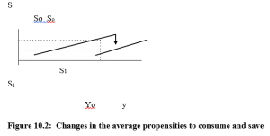
Figure 10.2: Changes in the average propensities to consume and save
Assume either a fall in interest rates or an increase in household wealth causes households to spend more (save less) of their income. The effect is illustrated in Figure 10.2. Prior to the change c0 is being spent and s0 is being saved from y0. After the change, c1 is being spent and s1 is being saved from y0. Note – the APC has risen (c0/y0 à c1/y0) while the APS has fallen
(s0/y0 à s1/y0).
Investment Function
The investment expenditure of firms (I) is the second component of aggregate demand in the two-sector model. Investment expenditure is defined as expenditure on output that is not for consumption in the current period. Capital investment is expenditure on plant and equipment while inventory investment is expenditure leading to increased stock levels. It is quite possible that firms could be engaging in unplanned inventory investment if, due to falling sales, there is an undesired accumulation of unsold stocks. This unplanned investment expenditure is included in GDP but is not included in aggregate demand. Changes in stock levels are the signal to firms to change their level of output and employment. If stock levels are falling due to rising demand, firms will tend to expand production whereas if stock levels are rising due to falling demand production is likely to be reduced.
Factors likely to influence the desired level of investment expenditure are: Ø interest rates;
- business confidence;
- the rate of change of income and expenditure.
The desired level of investment expenditure will be negatively related to changes in interest rates. Also the more confident firms are about future market conditions, the more willing they will be to invest in the present period. The accelerator theory suggests that the rate of change of income and expenditure has an important influence on the level of investment expenditure. Whatever the present level of income happens to be, the above factors may be exerting a positive or negative influence on the desired level of investment expenditure. It is assumed, unless otherwise stated, that the current desired level of investment expenditure is not influenced by the current level of income. This assumption is illustrated in Figure 10.3.
The horizontal investment function (I0) implies that the current level of income (Y) is not a factor influencing the desired level of investment expenditure. If there is an increase in the desired level of investment expenditure due to, say, a fall in interest rates, the investment schedule in Figure 10.3 will shift upwards and vice versa. From the point of view of the simple circular flow model of the economy investment expenditure is regarded as exogenously determined, i.e. it is not determined by variables which are themselves determined within the model.
The aggregate demand schedule for the two sector economy can be arrived at simply by adding the desired level of investment expenditure (I) to the desired level of consumption expenditure (C). This is illustrated in Figure 10.4.
As income rises aggregate demand (C + 1) rises due to the positive relationship between Y and C. The C + I line will have the same slope (MPC) as the consumption function and it is arrived at by simply adding the investment function of Figure 10.3 to the consumption function of Figure 10.1(a).
The level of output in the Keynesian circular flow model is determined by firms simply adjusting their production levels to satisfy the level of aggregate demand in the economy. If the aggregate demand for goods and services exceeds the current output of goods and services ( C + I > Y) then firms will expand production. If, on the other hand, aggregate demand is less than current output ( C + I < Y) firms adjust by cutting production. The equilibrium level of output is where aggregate demand is equal to the current level of output:
Y=C+I
[10.6]
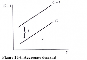
Figure 10.4: Aggregate demand
Equation (10.6) represents the equilibrium condition for a two-sector model of the economy. In equilibrium the realised outcomes (GDP measures) are equal to the planned measures (AD measures).
An alternative way of thinking of equilibrium is to focus on injections and withdrawals. Withdrawals from the circular flow are incomes earned but not passed on as expenditure on domestically produced goods and services. Injections into the circular flow are expenditures on domestically produced goods and services which are exogenously determined (coming from outside the system). In the two-sector model, savings represent a withdrawal while investment expenditure represents an injection. The income expenditure equilibrium (y = C + I) can be reformulated in terms of injections and withdrawals. We know that y = C + S. Substituting C + S for y in the equilibrium condition gives:
C+S = C+I or
S = I
[10.7]
Equation [10.7] tells us that the economy is in equilibrium when the level of injections (investment expenditure) is equal to the level of withdrawals (savings). Both equilibrium conditions are illustrated in Figure 10.5.
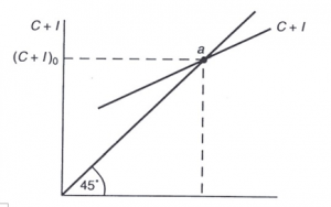
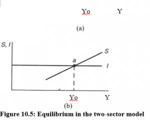
Figure 10.5: Equilibrium in the two-sector model
In Figure 10.5(a) the 45° line corresponds to the equation C + I = Y. Therefore any point on the 45° line satisfies the equilibrium condition for the economy. However the actual aggregate demand function for the economy (C + I) has a slope less than one ( = MPC) and therefore must intersect the 45° line. The point of intersection (a) represents the equilibrium for the economy with an equilibrium output of y o corresponding to the level of aggregate demand (C + I) 0. At output levels less than y 0 aggregate demand exceeds output so the economy will expand. At output levels greater than y 0 aggregate demand is less than output so the economy will contract.
Figure 10.5(a) is referred to as an ‘income/expenditure’ diagram. Figure 10.5(b) represents the corresponding ‘injections/withdrawals diagram ‘. These diagrams represent alternative ways of illustrating the equilibrium output of the economy which in both cases is y0. At output levels below y0 in Figure 10.5(b) injections exceed withdrawals causing the economy to expand whereas at output levels above y0 withdrawals exceed injections causing the economy to contract.
UNDEREMPLOYMENT EQUILIBRIUM
The point that Keynes was concerned to emphasise was that the equilibrium level of income was not necessarily the full employment level of income. It was possible for the economy to be in equilibrium but with high levels of unemployment (an underemployment equilibrium). This situation is illustrated in Figure 10.6.
C+I
Figure 10.6: Deflationary gap
The equilibrium level of output is Yo, but Yf is the required level of output if full employment is to be achieved. This economy is experiencing a deflationary gap. i.e. too little expenditure. The deflationary gap, indicates the amount of new expenditure that needs to be injected into the economy and is equal to the distance bc in both diagrams. .
The problem as Keynes saw it can be appreciated if we focus on the savings investment equilibrium (S = I). Decisions regarding the level of savings are being made by households while decisions regarding the level of investment are being made separately by firms. There was no reason to assume that these decisions would coincide at a full employment equilibrium. The point is illustrated in Figure 10.7.
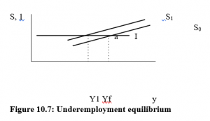
Figure 10.7: Underemployment equilibrium
Let’s assume that, starting at a full employment equilibrium (a), households decide to save more (spend less), causing the savings function to shift from So to S1. Unless firms spend more on investment, output will fall from Yf to yY1. But, according to Keynes, firms would be unlikely to increase investment at a time when demand and therefore sales were falling. Therefore the economy will move to an underemployment equilibrium at Y1. The classical economists believed that the increased savings represented an increase in loanable funds which would cause interest rates to fall and thus stimulate investment. Keynes, however, was more concerned with the blow to business confidence resulting from falling consumer demand.
The nature of the underemployment equilibrium illustrated in Figure 10.7 is of interest. Y1 is the equilibrium level of income following the increase in savings. However it is not like a micro-economics equilibrium where markets clear as a result of the equality between supply and demand. At Y1 in Figure 10.7 there is involuntary unemployment and therefore labour markets cannot be clearing. More workers are seeking employment than are being offered jobs.
Keynes argued that there was a need for the government to intervene in the economy to ensure that the level of aggregate demand was sufficient to generate full employment. However, sticking with our two-sector model which has no government, the only way aggregate demand can rise is if households decide to save less of their income (an autonomous increase in consumption expenditure) or if firms decide to raise investment expenditure. Either of these will result in an upward shift in the aggregate demand function.
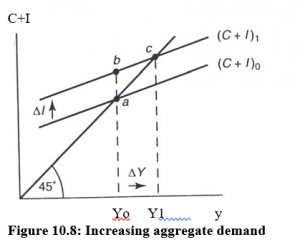
Figure 10.8: Increasing aggregate demand
Figure 10.8 illustrates with reference to an increase in investment expenditure. Assume the initial equilibrium Yo is an underemployment equilibrium. An exogenously determined change in investment expenditure shifts the aggregate demand function from (C + I)o to (C + I)1 – we are not concerned to explain the cause of this change but merely to trace the effect of it. The initial effect is for the economy to shift from point a to point b. However point b is not an equilibrium point (AD > Y0)’ the economy expands to the new equilibrium at point c with income equal to Y1. Certain features of this movement from Y0 to Y1 should be noted:
- In the simple circular flow model it is assumed that prices do not change. This fix price assumption means that the economy’s GDP expands in real terms (Section 9C) as a result of the increase in aggregate demand:
- .There are exogenous and induced changes in expenditure occurring. The increase in investment expenditure (exogenous) causes income to rise but this rise in income causes further induced changes in consumption expenditure (the movement from b to c).
- .Because of the exogenous and induced changes in expenditure the final change in income (AY) is greater than the initial change in investment expenditure (A1). This is known as the multiplier effect.
THE MULTIPLIER EFFECT
The Multiplier is the ratio of the total increase in national income to the initial increase. i.e.
| Multiplier =
|
Total Increase in National Income Initial increase in National Income |
Or it is a measure of the effect on total National Income of a unit change in some part of aggregate demand i.e. investments or government spending or exports.
An Initial increase in expenditure has a snowball effect, leading to more and more spending in the economy leading of a larger increase in National Income.
E.g. using the simple multiplier ( ) MPS __1
Where the MPS is the marginal propensity to save and MPC is the marginal propensity to consume.
If investment increases by 100,000 and MPC = 0.25, by how much does National Income increase?
Answer: ____MP1 = ________1 – MPC1 = 1_______ – 10.25 = ____0.75 1
National Income increases by 100,000 x ____0.75 1 = RWF133,000
De-multiplier: When there is a reduction in investments or government spending or exports, there is a bigger reduction in total national income because of the reverse multiplier.
Factors which affect MPS and MPC will affect the multiplier.
E.g: the age distribution of the population, The income distribution of the population, Expectations of the future.
Importance of the Multiplier
It is important because it means that an increase in one component of aggregate demand will increase national income by more than the initial increase.
So, if the government can boost spending initially (e.g. by increasing government spending or giving investment or export grants, or lowering interest rates) it can set off a general expansionary process.
In an open economy (i.e. one which trades with other countries) and where there is government intervention the multiplier becomes:
|
Open Economy Multiplier =
|
___________________1
MPS + MPT + MPM |
i.e. the multiplier effect is smaller the bigger are the withdrawals from the circular flow..
E.g. – if MPS = 10%, MPM = 45% and MPT = 25%
____1
The “Simple” multiplier = 0.1 = 10.
But the open economy multiplier = _________________0.1 + 0.45 + 0.25 1 = 1.25
Limitations of the Multiplier
- If there is full employment, any increase in demand will be inflationary. (But can use the “de-multiplier” effect here).
- If the withdrawals (i.e. leakages) from the circular flow, savings, taxation or imports, are high the multiplier will be very small so “pump priming” will have little effect.
- There may be a long-term lapse before the benefits of the multiplier take effect. (So it is no good as a short-term solution to unemployment or inflation).
- The consumption function in modern times is volatile therefore the effects of the multiplier are also unpredictable.
- If the government tries to increase spending it can lead to other problems in the economy. The extra spending must be financed. If the government raises taxes, the multiplier will be lower and people may work less hard. If it borrows the money it can lead to high national debt problems and cause interest rates to rise.
The Accelerator Principal
This states that if the RATE of increase in consumer goods is rising, there must be an even faster rate of increase in investment by firms, so as to boost production capacity enough to meet the higher demand.
[There is also a “decelerator” effect where when National Income is falling the percentage drop in investment is even faster than the rate of fall in consumption.]
The accelerator principle means that;
- National Income remains high only as long as investments are high, and
- investment is high only so long as income and consumption are RISING.
So, as National Income approaches its peak level (boom) as determined by available capacity, NEW investment will fall towards zero, reducing aggregate demand and hence National Income.
This decelerator effect will be compounded by the de-multiplier and national income will fall sharply.
Investment and the Business Cycle
An investment: committing resources (i.e. factors) to a long-term project with a view to earning a satisfactory return over the period of the project.
The six main factors that influence the volume of investment are:
The expected return from investments
An investment involves the acquisition of more buildings, machinery, plant and equipment (i.e. NET investments)
Firms should go on adding to their capital so long as the marginal efficiency of capital (MEC) exceeds the marginal cost of the extra capital (i.e. the interest rate).
In other words, the expected rate of return must at least equal the required rate of return (i.e. the MC of investment).
- Risk, Confidence and expectations about future prospects.
Investment projects are long-term ventures; it takes several years to reap the full return. So there is a risk to investment because the future is uncertain.
If confidence is high (i.e. there are good expectations about the future) investment will increase. The bigger the risk or perceived risk the lower will be investment. Risk is bigger with a new market or a new product.
- New technology boosts investments because:
- it can reduce the unit costs of production (by enabling the factors of production to be more productive.) This increases profitability and supply will increase as firms invest more to achieve lower costs and remain competitive.
- new technology leads to new types of goods which stimulate consumer demand and firms will invest more to meet this extra demand.
- The Accelerator principle/changes in income.
- Government Grants and Subsidies.
Governments can encourage investment by giving grants and subsidies.
Government Grants are generally “regional” i.e. aimed at areas of high unemployment or “export related” to encourage firms to export or “innovative” to boost R & D. In terms of Agriculture, grants may be aimed at food production to make the country less reliant on imports.
They often effect decisions on where to invest rather than whether or not to invest.
Business Cycles
These are the continual sequence of rapid growth in national income, followed by a slowdown in growth and then a fall in national income (recession) which eventually changes back to growth and so on.
A trade cycle or business cycle has four phases (period of the cycle seven years)
| Characteristics | ||||||
| 1. | Depression | (a) Heavy Unemployment | ||||
| (b) Low consumer demand | ||||||
| (c) Over Capacity (unused capacity in production) | ||||||
| (d) Prices stable, or even falling | ||||||
| (e) Business Profits Low | ||||||
| (f) Business Confidence in the future Low | ||||||
| 2. | Recovery | (a) Investment picks up. | ||||
| (b) Employment rises | ||||||
| (c) Consumer spending rises | ||||||
| (d) Profits rise | ||||||
| (e) Business Confidence Grows | ||||||
| (f) Prices stable, or slowly rising | ||||||
| 3. | Boom | (a) Consumer Spending Rising fast | ||||
| (b) Output capacity reached: labour shortages occur (c) Output can only be increased by new labour-saving investment (technology). (d) Investment spending high. (e) Increases in demand now stimulate price rises. (f) Business Profits high |
||||||
| 4. | Recession | (a) Consumption falls off
(b) Many investments suddenly become unprofitable and new investments falls |
||||
| (c) Production falls | ||||||
| (d) Employment falls | ||||||
| (e) Profits fall, some businesses fail | ||||||
| (f) Recession can turn into severe depression | ||||||
Explanation of Business Cycles 1. Pre Keynesian Theories Different steps in the cycle:
Recovery
- Investment begins to rise because;
- interest rates have fallen
- cost of factors have fallen
- new technologies
- expectations
- Once investments start to rise, more labour will be employed (to make the capital equipment that is being invested in). This increases income, leading to higher consumer spending and therefore still more investment which again boosts demand, etc.
The increase in demand eventually pushes up prices.
- Eventually the upswing flattens out – because of over-investment during the boom. This surplus capacity eventually leads to redundancies and this unemployment causes a fall in income and consumption. (iv) The accelerator principle increases this cyclical effect.
Keynes’ theory: Multiplier – Accelerator Theory
The combination of the multiplier and accelerator explain the upswings and downswings in the business cycle.
The Paradox of Thrift
This illustrates the workings of a “de-multiplier” in a situation where savings and investments are temporarily out of balance.
All income that is saved is not necessarily invested – some savings are held as money (i.e. cash or near cash).
- If this is so a rise in savings will cause a fall in consumption which may cause businesspeople to reduce investment.
- This fall in investment, through the multiplier, causes greater reductions in national income.
- The fall in National income, means households have smaller incomes and so save less. Paradox of Thrift: Greater savings without greater investment end with smaller incomes and smaller savings.
Policies on Investment – Government and the Trade Cycle
The government can try to influence the trade cycle – moderate the upswings and downswings – using management.
- Encourage new investment (grants and subsidies) or itself invests
- Increase Government spending by borrowing or reduce taxes.
- Encourage exports with subsidies and discourage imports (tariffs, quotas etc.) If demand is too strong, government policies would be the opposite.
Government can influence investment by:
- Controlling interest rates
- Grants and subsidies to encourage investment
- Boost business confidence – announcing and achieving policy objectives for growth and development.
- Encourage technological progress, Research and development.
- Control the money supply to change consumption (f) Direct Government Spending (g) Keeping tax low.
Importance of Investment
- Public sector investment has valuable spin-offs – better infrastructure, telecommunications etc.
- Investment represents consumption foregone now to increase the capacity to produce and consume in the future – it shapes the future growth and development of nations.
- It is vital determinant of the economies long-term growth rate.
Financing of Investment Private sector Investment
- Retained profits
- New share issues
- Borrowing
Public Sector Investment
- higher taxation
- Borrowing
- Bond issues
Note public sector investment can “crowd out” private investment.
It can be shown that for Figure 10.8 :
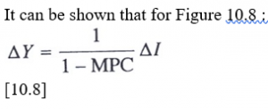
[10.8]
where 1/1- MPC is the multiplier. The multiplier effect is easily illustrated using the savingsinvestment diagram. In Figure 10.9 the initial equilibrium is yo. The MPC is assumed to be 0.8.
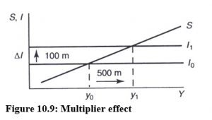
Figure 10.9: Multiplier effect
(i.e. MPS = 0.2). Investment expenditure rises by RWFl00m. The value of the multiplier is 5 (i.e. 1/1- 0.8). The final change in income is RWF500m.
∆Y= 1 – 1 0.8 x RWF100m = RWF500m
Note as income rises from Yo to Y1 there is an induced increase in savings. Income rises until the new level of savings is equal to the higher level of investment. The multiplier effect results from successive (but diminishing) rounds of expenditure following the initial increase in expenditure. Initially investment expenditure rises by RWF100m causing incomes to rise by the same amount. However because MPC = 0.8, RWF80m of this increased income will be spent causing incomes to rise by an additional RWF80m. RWF64m of this additional change will be spent. ..and so on.
THE PARADOX OF THRIFT
The paradox of thrift relates to the possibility of households intending to save more (or less) but actually ending up saving less (or more). In Figure 10.10 it is assumed that the level of investment expenditure is positively related to the level of income (as illustrated by the upward slope).
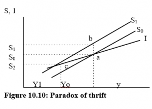
Figure 10.10: Paradox of thrift
The initial equilibrium is at point a with income level of y0 and s0 being saved. Households decide (for whatever reason) to save more and therefore spend less of their incomes. This is indicated by the upward shift in the savings function from S0 to S1. Because the increase in savings represents a fall in aggregate demand, the equilibrium level of income falls from y0 to y1 (point c represents the new equilibrium). Although the savings ratio has increased, the overall level of savings has fallen due to the fall in the level of income. Households had intended saving an amount s1 from y0 but end up saving an amount s2 from y1, i.e. the level of savings has fallen despite the original intention to increase savings.