
. GOVERNMENT POLICIES AND OBJECTIVES
Governments play a major role in all modern economies. Public procurements – government expenditure on defence, education, health, transport, etc. – represent a major claim on the economic resources of society. Government expenditure is therefore an important component of aggregate demand in the economy.
Governments also pursue broader policy objectives. Although the priorities can shift depending on circumstances, the following are the well established objectives of macroeconomic policy: Ø Full employment;
- Low inflation;
- Economic growth;
- Satisfactory balance of payments;
- Redistribution of income in society.
The problem for governments is that these objectives are not always mutually consistent. Conflicts can emerge, for example, in trying simultaneously to achieve full employment and low inflation, or in trying to achieve economic growth while having generous policies for redistributing income from rich to poor. Priorities will have to be established and a trade-off between objectives may be necessary.
To achieve their macroeconomic objectives governments must formulate appropriate policies. Macroeconomic policies tend to be classified under two broad headings:
- Fiscal policy: using the powers of taxation and government expenditure to achieve objectives.
- Monetary policy: using interest rates and the money supply to achieve objectives.
In the context of the simple Keynesian circular flow model, the focus is on the use of fiscal policy to achieve the full employment objective. Being a fixed price model, it is clearly inadequate for analysing issues concerning inflation.
CLOSED ECONOMY MODEL
By including a government in the model we need to take account of an additional withdrawal from and injection into the circular flow of income and expenditure:
- Taxation (T) represents a withdrawal from the circular flow. It represents income earned which is passed to the government rather than passed on as expenditure on domestically produced goods and services.
- Government Expenditure (G) represents an injection of expenditure into the circular flow.
The fiscal policy being pursued by the government will be reflected in the annual budget. With regard to the impact of the budget on aggregate demand there are three possible scenarios:
- Balanced budget: (G = T) – injections equal withdrawals implying a neutral effect on aggregate demand;
- Budget deficit: (G > T) – injections exceed withdrawals causing aggregate demand to increase (‘expansionary budget’);
- Budget surplus: (G < T) – withdrawals exceed injections causing aggregate demand to decrease (‘contractionary budget’).
A budget deficit will force the government to seek additional (besides taxation) sources of finance. Typically a budget deficit can be expected to result in a public sector borrowing requirement (PSBR). Annual borrowing in turn contributes to the national debt, which is simply all outstanding (unredeemed) public sector debt. A budget surplus may be used for public sector debt repayment (PSDR) which represents a reduction in the national debt.
In practice governments have additional sources of finance besides taxation and borrowing. These include the proceeds of privatisation or the profits of state sector enterprises. However these sources are either one-off or relatively insignificant and will be ignored in the following analysis.
There are three components of aggregate demand (AD) in the closed economy:
AD = C + I + G [11.1]
Government expenditure (G) is exogenously determined in that its level cannot be explained by reference to the economic variables of the model. The level of G depends on the ideological make-up of the government which may be sympathetic to relatively high or relatively low levels of public expenditure.
Because taxation exists, it is necessary to distinguish between the gross factor incomes of households (Y) and the disposable income of households (Yd). Disposable income is what remains after taxes have been deducted:
Yd = Y – T [11.2]
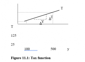
Figure 11.1: Tax function
If we assume for simplicity that all taxes are direct, i.e. taken directly from gross income, then the level of taxation (T) depends on two things: the rate of tax and the level of income (Y).
Taxation is therefore endogenously determined. Given the rate of tax the amount of tax is determined by the level of income. As income rises the level of tax rises and vice versa. Figure 11.1 illustrates a simple tax function.
As gross incomes rise tax revenue increases. The marginal rate of tax (MRT) which is the rate of tax on an additional RWF1 earned, is indicated by the slope of the line (A T / A Y). If we assume a simple tax function of the form T = 0.25Y then for Y= RWF100, T= RWF25 and for Y= RWF500, T= 125, etc. The proportion of any change in income that is taken by the government in tax (AT/AY) is sometimes referred to as the marginal propensity to tax (MPT). Households must now decide how much of their disposable incomes (rather than gross incomes) to spend or save. A given marginal propensity to consume from disposable income (MPC) will mean a lower marginal propensity to consume from gross income (MPCg).
Example Assume:
- All income is taxed at a rate of 25% (MRT = 0.25)
- Households spend 80% of any additional disposable income (MPC = 0.8) and save 20% (MPS = 0.2). Then
T = O.25Y
Yd = Y-T = Y-O.25Y = O.75Y
∆C = O.8∆Yd
= O.8(0.75)∆Y = O.6∆Y
i.e. given a 25% marginal tax rate, a marginal propensity to consume from disposable income of 0.8 implies a marginal propensity to consume from gross income of 0.6.
The aggregate demand function for the closed economy can be illustrated as in Figure 11.2.
Aggregate demand at any given level of income is arrived at by simply adding the relevant levels of C, I and G. Both I and G are assumed to be independent of
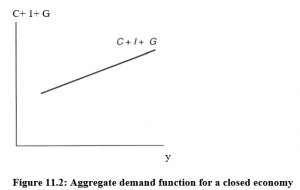
Figure 11.2: Aggregate demand function for a closed economy
the level of income whereas C is positively related to it. The slope of the aggregate demand function is ∆C/∆Y (i.e. MPCg). The slope of the line in Figure 11.2 is flatter than that in Figure 10.1 (a) due to the inclusion of taxation. It follows that the multiplier effect is weakened by the inclusion of taxation. The formula for the multiplier (k) is now:
Quite simply the greater the scope for withdrawals from the circular flow the lower the proportion of any change in gross income that is passed on as expenditure thus reducing the multiplier effect.
Equilibrium in the Closed Economy
The equilibrium condition for the closed economy is:
Y=C+I+G
[11.4]
When the sum of the desired levels of expenditure in the economy ( C + I + G) is equal to the value of output (Y) being produced in the economy, there will be no tendency for economic expansion or contraction. The equilibrium can be illustrated using an income expenditure diagram as in Figure 11.3.
The equilibrium level of income is determined at the point where the aggregate demand function intersects the 45° line. This is at point a in Figure 11.3 with an equilibrium income of Yo.
An alternative formulation of the equilibrium condition is in terms of injections and withdrawals.
S+T=I+G [11.5]
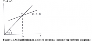
Figure 11.3: Equilibrium in a closed economy (income/expenditure diagram)
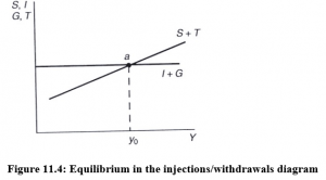
Figure 11.4: Equilibrium in the injections/withdrawals diagram
As both withdrawals (S ,T) are positively related to the level of income and both injections (I,G) are independent of the level of income (exogenous) this equilibrium condition can be illustrated as in Figure 11.4.
The equilibrium level of income (Yo) is determined at the point of intersection of the injections and withdrawals functions (point a).
ACTIVE FISCAL POLICY
As we have seen, Keynes was pessimistic about the capacity of an unregulated free market economy to generate a full employment equilibrium. The Keynesian analysis was developed in the period between the two World Wars, a period of global economic and political instability. The depression of the early 1930s was characterised by mass unemployment in Europe and in the USA. Not a time when one’s confidence in the free market system was likely to be strengthened.
Because governments must raise taxes to finance expenditure on such things as defence, education, etc., a fiscal policy of some sort is unavoidable. However the traditional policy of governments was to pursue ‘fiscal rectitude’. This meant keeping taxation and therefore government expenditure as low as possible while balancing the budget. What Keynes argued was that governments should have an active fiscal policy with a view to influencing the overall level of aggregate demand in the economy. If the economy was experiencing a deflationary gap the government should either raise government expenditure or lower taxes or some combination of both. Figure 11.5 illustrates an economy which is initially in an underemployment equilibrium (point a).
By increasing expenditure by an amount equal to AG the government can shift the aggregate demand function from ( C + I + G)o to ( C + I + G) I. A new equilibrium is achieved at point b which is a full employment equilibrium. Note because of the multiplier effect the government does not have to raise G by the required increase in Y
∆Y = 1 ∆G [11.6]
1− MPC (1− MRT)
Example
Assume the government needs to raise the level of output by RWF1000m (∆Y= RWF1000m) to achieve full employment. The MPC = 0.8 and the MRT = 0.25.
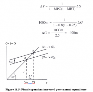
Figure 11.5: Fiscal expansion: increased government expenditure
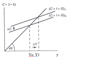
Figure 11.6: Fiscal expansion: reduction in taxation
Therefore if the government increases expenditure (∆G) by RWF400m income will rise by RWF1000m.
If instead of increasing government expenditure the government reduced taxes it could stimulate household expenditure (C) by raising household disposable income (Yd). However C will not initially increase by the full reduction in taxation as only some proportion (the MPC) will be spent while some proportion (the MPS) is saved. The initial increase in consumption will be equal to MPC times ∆T. Figure 11.6 illustrates fiscal expansion by way of a tax reduction.
In Figure 11.6 AC = MPC ∆T. The multiplier effect resulting from a reduction in taxation will be less than the multiplier effect for an increase in government expenditure:

change in taxes (∆7). Because the taxation multiplier [11.7] is less than the government expenditure multiplier (11.6) it is possible to achieve a balanced budget multiplier effect. If government raises taxation and expenditure by an equal amount, the increase in taxes will reduce income by a smaller amount than the increase in expenditure will raise it. The overall effect, therefore, will be positive. The net effect is the result of the government spending income that households had in fact been saving.
OPEN ECONOMY MODEL
In an open economy we must take account of international trade. Exports are domestically produced goods the demand for which originates abroad. Foreign expenditure on the economy’s exports (X) represents an injection of income and expenditure into the domestic economy. Imports are foreign produced goods the demand for which originates in the domestic economy. Domestic expenditure on imports (M) represents income earned which is not passed on as expenditure on domestic production and is therefore a withdrawal from the circular flow.
The value of imports will depend on:
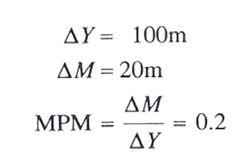
The level of domestic income (Y) – as income rises more will be spent. It is assumed that some of this additional expenditure will go on imports The marginal propensity to import (MPM) is the proportion of any change in income that is spent on imports
Example
- The real exchange rate (Section 14A) -the competitiveness of domestic goods and services relative to foreign ones will influence consumers’ purchases. Competitiveness depends on the nominal exchange rate (Section 14A) and domestic prices relative to foreign prices.
The value of exports will depend on:
- The level of world income – if income and expenditure are rising in the economies of trading partners this will lead to an increase in demand for exports (for example if the Kenyan economy is booming this will stimulate demand for Rwandan exports).
- The real exchange rate – if domestically produced goods and services lose competitiveness on world markets, exports will be adversely affected and vice versa.
- In the completed circular flow model there are three injections (G, I, X) and three withdrawals (S, T, M) as illustrated in Figure 11.7. All the injections are exogenously determined, i.e. their levels are determined by factors not included in the model. The withdrawals are endogenously determined as the level of domestic income (Y) has a positive influence on all of their levels.
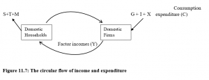
Figure 11.7: The circular flow of income and expenditure
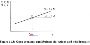
Figure 11.8: Open economy equilibrium: (injections and withdrawals)
The economy will be in equilibrium with no tendency for output to expand or contract when the sum of injections equals the sum of withdrawals:
S+T+M=G+I+X [11.8]
This equilibrium condition can be illustrated in an injections/withdrawals diagram as in Figure 11.8.
The economy is in equilibrium at point a where the injections line intersects the withdrawals line with income Yo.
Aggregate Demand in an Open Economy
The aggregate demand for domestically produced goods and services in an open economy is:
AD = C+I+G+ (X-M) [11.9]
The equilibrium condition is that total desired expenditure be equal to the value of domestic output:
Y = C+I+G+(X-M) [11.10]
This equilibrium condition is an alternative formulation of Equation [11.8] and is illustrated in Figure 11.9.
Equilibrium is at point a with income at Yo. The aggregate demand function in Figure 11.9 has a slope which is flatter than that of Figure 11.2. This is because imports are positively related to the level of domestic income (i.e. endogenously determined) and are included in the function with a negative sign. It follows that the multiplier effect is weakened when we move from a closed to an open economy.
The formula for the open economy multiplier is:
k = 1
1− MPC (1− MRT) + MPM
Example MPC = 0.8
MRT = 0.25
MPM = 0.2
k = = = 1.67
Clearly the multiplier effect, resulting from any injection of demand into the economy, will be weaker the higher is the MPM. Figure 11.10 illustrates the multiplier effect with respect to a change in government expenditure (∆G). Note, the relationship between ∆G and ∆Y depends on the open economy multiplier.
∆Y = 1 = ∆G
1− MPC (1− MRT) + MPM
We can conclude that fiscal policy in an open economy will have less effect on economic activity than in a closed economy. The higher the MPM, the smaller the multiplier and the less impact policy will have.
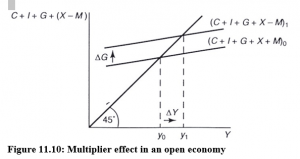
Figure 11.10: Multiplier effect in an open economy
LIMITATIONS OF THE SIMPLE KEYNESIAN MODEL
The simple Keynesian model of income determination, developed in this and the previous chapter, explains the level of economic activity by reference to the level of aggregate demand. If there is unemployment in the economy government can remove it by raising aggregate demand by means of fiscal policy. All economic models simplify reality with a view to clarifying key relationships. All resort to the ceteris paribus assumption in order to make conditional predictions. For example, ‘if aggregate demand is raised, all else being equal, the result will be increased economic activity’ is the conditional prediction of the simple Keynesian model.
Models can be criticised if the assumptions are wrong or key economic relationships are being left out so that either way the predictions are unreliable. The main weakness of a simple circular flow model is the absence of a monetary system. It focuses on production to supply markets for goods and services but has nothing to say about money. Because monetary issues are outside the scope of the model, it lacks the capacity to explain the following:
The Crowding Out Effect:
An increase in government expenditure may lead to a fall in private sector expenditure (‘crowding out’). For example, assume the government is pursuing an expansionary fiscal policy and is borrowing funds in the capital markets to finance a budget deficit. If this has the effect of raising interest rates then private sector investment expenditure and consumption expenditure are likely to fall. The crowding out effect calls into question the government’s ability to control the level of aggregate demand.
Stagflation:
This is a situation where unemployment and inflation are simultaneously rising. The simple model has a ‘fix price’ assumption. We can interpret this to mean that, if unemployment exists and aggregate demand rises, real output rather than the price level will rise. If, however, the economy is fully employed and aggregate demand continues to rise, then as output cannot rise, inflation will occur. In the simple model, inflation can only be due to too much demand in the economy. It follows that simultaneously rising inflation and unemployment are precluded by the model. Stagflation was a widespread problem in the global economy in the 1970s and was a major factor leading to a loss of confidence in Keynesian economics.
Other problems include.
The Nature of Unemployment:
The Keynesian model has a one-dimensional view of the cause of unemployment. The model explains unemployment by reference to the level of aggregate demand. If the latter is too low, unemployment will be the result. However, unemployment may have a number of causes. If so, simply increasing aggregate demand may not be an adequate policy.
Openness of Modern Economies:
We have seen that fiscal policy may be relatively ineffective with regard to influencing economic activity if there is a high marginal propensity to import. Modern economies are much more open than was the case when Keynes was developing his analysis. Clearly small open economies (particularly with high marginal rates of tax) will have relatively weak multiplier effects and therefore fiscal policy as prescribed by Keynes will be correspondingly weakened.