
INTRODUCTION
In discussing the capital budgeting techniques, we have so far assumed that the proposed investment projects do not involve any risk. This assumption was made simply to facilitate the understanding of the capital budgeting techniques. In real-world situation, however, the firm in general and its investment projects in particular are exposed to different degrees of risk. What is risk? How can risk be measured and analysed in the investment decisions?
NATURE OF RISK
Risk exists because of the inability of the decision maker to make perfect forecasts. Forecasts cannot be made with perfection or certainty since the future events on which they depend are uncertain. An investment is not risky if we can specify a unique sequence of cash flows for it. But the whole trouble is that cash flows cannot be forecast accurately, and alternative sequences of cash flows can occur depending on the future events. Thus, risk arises in investment evaluation because we cannot anticipate the occurrence of the possible future events with certainty and, consequently, cannot make any correct prediction about the cash flow sequence. To illustrate, let us suppose that a firm is considering a proposal to commit its funds in a machine, which will help to produce a new product. The demand for this product may be very sensitive to the general economic conditions. It may be very high under favourable economic conditions and very low under unfavourable economic conditions. Thus, the investment would be profitable in the former situation and unprofitable in the latter case. But, it is quite difficult to predict the future state of economic conditions. Because of the uncertainty of the economic conditions, uncertainty about the cash flows associated with the investment derives.
Industry factorsThis category of events may affect all companies in an industry. For example, companies in an industry would be affected by the industrial relations in the industry, by innovations, by change in material cost, etc.
A large number of events influence forecasts. These events can be grouped in different ways. However, no particular grouping of events will be useful for all purposes. We may, for example, consider three broad categories of the events influencing the investment forecasts:1 General economic conditions This category includes events which influence the general level of business activity. The level of business activity might be affected by such events as internal and external economic and political situations, monetary and fiscal policies, social conditions, etc.
Company factorsThis category of events may affect only the company. The change in management, strike in the company, a natural disaster such as flood or fire may directly affect a particular company.
In formal terms, the risk associated with an investment may be defined as the variability that is likely to occur in the future returns from the investment. For example, if a person invests, say `20,000 in short-term government bonds, which are expected to yield 9 per cent return, he can accurately estimate the return on the investment. Such an investment is relatively risk free. The reason for this belief is that government will not fail and will pay interest regularly and repay the amount invested. It is for this reason that the rate of interest paid on government securities, such as short-term treasury bills, is the risk-free rate of interest. Instead of investing `20,000 in government securities, if the investor purchases the shares of a company, then it is not possible to estimate future return accurately. The return could be negative, zero or some extremely large figure. Because of the high degree of the variability associated with the future returns, this investment would be considered risky.
Risk is associated with the variability of future returns of a project. The greater the variability of the expected returns, the riskier the project. Risk can, however, be measured more precisely. The most common measures of risk are standard deviation and coefficient of variations.
STATISTICAL TECHNIQUES FOR RISK ANALYSIS
Statistical techniques are analytical tools for handling risky investments.2 These techniques, drawing from the fields of mathematics, logic, economics and psychology, enable the decision maker to make decisions under risk or uncertainty.3
The concept of probability is fundamental to the use of the risk analysis techniques. How is probability defined? How are probabilities estimated? How are they used in the risk analysis techniques? How do statistical techniques help in resolving the complex problem of analysing risk in capital budgeting? We attempt to answer these questions in this section.
Probability Defined
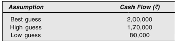
Probability may be described as a measure of someone’s opinion about the likelihood that an event will occur. If an event is certain to occur, we say that it has a probability of one of occurring. If an event is certain not to occur, we say that its probability of occurring is zero. Thus, probability of all events to occur lies between zero and one. A probability distribution may consist of a number of estimates. But in the simple form it may consist of only a few estimates. One commonly used form employs only the high, low and best guess estimates, or the optimistic, most likely and pessimistic estimates. For example, the annual cash flows expected from a project could be `2,00,000 or `1,70,000 or `80,000:
The most crucial information for the capital budgeting decision is the forecast of future cash flows. A typical forecast is single figure for a period. This is referred to as ‘best estimate’ or ‘most likely’ forecast. But the questions are: To what extent can one rely on this single figure? How is this figure arrived at? Does it reflect risk? In fact, the decision analysis is limited in two ways by this single figure forecast. Firstly, we do not know the chances of this figure actually occurring, i.e., the uncertainty surrounding this figure. In other words, we do not know the range of the forecast and the chance or the probability estimates associated with figures within this range. Secondly, the meaning of best estimates is not very clear. It is not known whether it is mean, median or mode. For these reasons, a forecaster should not give just one estimate, but a range of associated probability—a probability distribution.
It can easily be seen that this is an improvement over the single figure forecast. But still some more information can be disclosed. What does the forecaster feel about the occurrence of these estimates? Are these forecasts likely equal? The forecast should describe more accurately his degree of confidence in his forecasts; that is, he should describe his feelings as to the probability of these estimates occurring.4 For example, he may assign the following probabilities to his estimates:
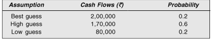
The forecaster considers the chance or probability of the annual cash flows being either `2,00,000 (maximum) or `80,000 (minimum) at 20 per cent each. There is a 60 per cent probability that annual cash flows may be `1,70,000. The additional information provided by the forecaster is useful in assessing more clearly the impact of a variable, which may assume different values on the profitability of an investment. A pertinent question is: How to obtain probability distributions?
Assigning probability
The classical probability theory assumes that no statement whatsoever can be made about the probability of any single event. In fact, the classical view holds that one can talk about probability in a very long-run sense, given that the occurrence or non-occurrence of the event can be repeatedly observed over a very large number of times under independent identical situations. Thus, the probability estimate, which is based on a very large number of observations, is known as an objective probability.
Risk and Uncertainty
The classical concept of objective probability is of little use in analysing investment decisions because these decisions are non-repetitive and hardly made under independent identical conditions over time. As a result, some people opine that it is not very useful to express the forecaster’s estimates in terms of probability. However, in recent years another view of probability has revived, that is, the personalistic view, which holds that it makes a great deal of sense to talk about the probability of a single event, without reference to the repeatability, long-run frequency concept. It is perfectly valid, therefore, to talk about the probability of rain tomorrow, the probability of sales reaching a certain level next year, or the probability that earnings per share will exceed `2.50 next year, or five years hence.5 Such probability assignments that reflect the state of belief of a person rather than the objective evidence of a large number of trials are called personal or subjective probabilities.
Risk is sometimes distinguished from uncertainty. Risk is referred to a situation where the probability distribution of the cash flow of an investment proposal is known. On the other hand, if no information is available to formulate a probability distribution of the cash flows the situation is known as uncertainty. Most financial authors do not recognize this distinction and use the two terms interchangeably. We too follow this approach.
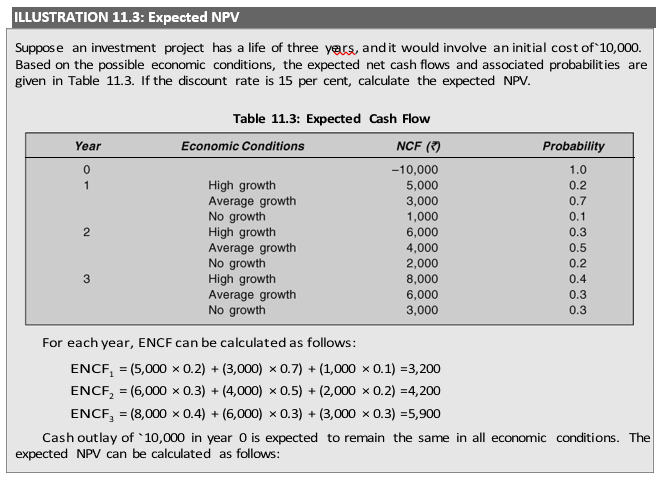
Expected Net Present Value
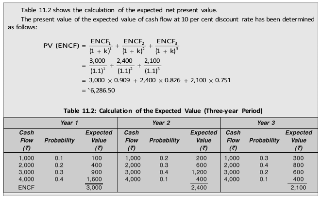
Once the probability assignments have been made to the future cash flows, the next step is to find out the expected net present value. The expected net present value can be found out by multiplying the monetary values of the possible events (cash flows) by their probabilities. The following equation describes the expected net present value.
Expected net present value = Sum of present values of expected net cash flows

where ENPV is the expected net present value, ENCFt expected net cash flows (including both inflows and outflows) in period t and k is the discount rate. The expected net cash flow can be calculated as follows:
![]()
where NCFjt is net cash flow for jth event in period t and Pjt probability of net cash flow for jth event in period t.
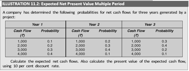
Instead of one-year cash flow estimates if we have cash flow estimates for several years, the mechanism for calculating the expected value just described can be simply extended.

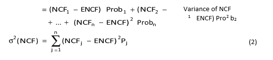
Variance or Standard Deviation: Absolute Measure of Risk
Although, through the calculation of the expected net present value, risk is explicitly incorporated into the capital budgeting analysis, yet a better insight into the risk analysis will be obtained if we find out the dispersion of cash flows, i.e., the difference between the possible cash flows that can occur and their expected value. The dispersion of cash flow indicates the degree of risk. A commonly used measure of risk is the standard deviation or variance. Simply stated, variance measures the deviation about expected cash flow of each of the possible cash flows. Standard deviation is the square root of variance. The formulae to calculate variance and standard deviation are as:
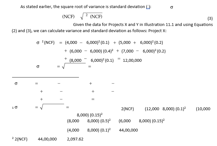
The calculation of standard deviation clearly shows that Project Y is riskier as it has a higher standard deviation. Had the expected net present values of the two projects been the same, on the basis of the standard deviation as a measure of risk, Project X would have been favoured. But the decision maker is in a dilemma because Project Y not only has a larger expected net present value, but also a larger standard deviation as compared to Project X.
2(NCF) 12,00,000 1,095.45
Project Y:
To resolve such problems, instead of analysing risk in absolute terms, it may be measured in relative terms.
Coefficient of Variation: Relative Measure of Risk
A relative measure of risk is the coefficient of variation. It is defined as the standard deviation of the probability distribution divided by its expected value:
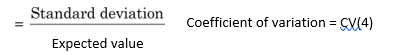
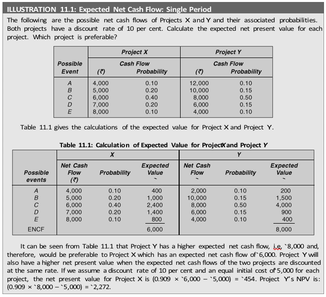
The coefficient of variation is a useful measure of risk when we are comparing the projects which have (i) same standard deviations but different expected values, or (ii) different standard deviations but same expected values or (iii) different standard deviations and different expected values. In Illustration 11.1, Project X has an expected value of `6,000 and a standard deviation of `1,095.45, while Project Y has an expected value of `8,000 and a standard deviation of `2,097.62. Intuitively, Project Y may be preferred because of the larger expected net present value. But it is more risky as compared to Project X. This is verified by calculating the coefficients of variation for the two projects. The coefficient of variation for Project X is (1,095.45/6,000) = 0.1826, while for Project Y it is (2,097.62/8,000) = 0.2622.
Whether Project X or Project Y should be accepted will depend upon the investor’s attitude towards risk. He would prefer Project Y if he is ready to assume more risk in order to obtain a higher expected monetary value. In case he has a great aversion to risk, he would accept Project X for it is less risky.
Check Your Concepts
- Define the concept of risk. Is it different from uncertainty?
- What factors cause investment uncertainty?
- Define probability. How does objective probability differ from subjective probability?
- How is expected present value calculated?
- What are the statistical measures of risk and how are they calculated?
TECHNIQUES OF RISK ANALYSIS
A number of techniques to handle risk are used by managers in practice. They range from simple rules of thumb to sophisticated statistical techniques.6 The following are the popular, non-conventional techniques of handling risk in capital budgeting:
Payback
Risk-adjusted discount rate
Certainty equivalent
These methods, as discussed ahead, are simple, familiar and partially defensible on theoretical grounds. However, they are based on highly simplified and, at times, unrealistic assumptions. They fail to take account of the whole range of the effect of risky factors on the investment decision making.
Payback
Payback is one of the oldest and commonly used methods for explicitly recognizing risk associated with an investment project. This method, as applied in practice, is more an attempt to allow for risk in capital budgeting decision rather than a method to measure profitability. Business firms using this method usually prefer short payback to longer ones, and often establish guidelines that a firm should accept investments with some maximum payback period, say three or five years.
The merit of payback is its simplicity. Also, payback makes an allowance for risk by (i) focusing attention on the near-term future and thereby emphasizing the liquidity of the firm through recovery of capital, and (ii) by favouring short-term projects over what may be riskier, longer-term projects.7
Further, even as a method for allowing risks of time nature, it ignores the time value of cash flows. For example, two projects with, say, a four-year payback period are at very different risks if in one case the capital is recovered evenly over the four years, while in the other it is recovered in the last year. Obviously, the second project is more risky. If both cease after three years, the first project would have recovered three-fourths of its capital, while all capital would be lost in the case of second project. Given the uncertainty element, it may well be that a four-year payback period based on fairly certain estimates might be preferred to a three-year payback period, calculated with very uncertain estimates.
It should be realized, however, that the payback period, as a method of risk analysis, is useful only in allowing for a special type of risk—the risk that a project will go exactly as planned for a certain period and will then suddenly cease altogether and be worth nothing. It is essentially suited to the assessment of risks of time nature. Once a payback period has been calculated, the decision maker would compare it with his own assessment of the projects likely, and if the latter exceeds the former, he would accept the project. This is a useful procedure, and economic only if the forecasts of cash flows associated with the project are likely to be unimpaired for a certain period. The risk that a project will suddenly cease altogether after a certain period may arise due to reasons such as civil war in a country, closure of the business due to an indefinite strike by the workers, introduction of a new product by a competitor which captures the whole market and natural disasters such as flood or fire. Such risks undoubtedly exist but they, by no means, constitute a large proportion of the commonly encountered business risks. The usual risk in business is not that a project will go as forecast for a period and then collapse altogether, rather the normal business risk is that the forecasts of cash flows will go wrong due to lower sales, higher cost, etc.8
Risk-Adjusted Discount Rate
For a long time, economic theorists have assumed that, to allow for risk, the businessman required a premium over and above an alternative, which was risk free. Accordingly, the more uncertain the returns in the future, the greater the risk and the greater the premium required. Based on this reasoning, it is proposed that the risk premium be incorporated into the capital budgeting analysis through the discount rate. That is, if the time preference for money is to be recognized by discounting estimated future cash flows, at some risk-free rate, to their present value, then, to allow for the riskiness of those future cash flows a risk premium rate may be added to risk-free discount rate. Such a composite discount rate, called the riskadjusted discount rate, will allow for both time preference and risk premium and will be a sum of the risk-free rate and the risk-premium rate reflecting the investor’s attitude towards risk. The risk-adjusted discount rate method can be formally expressed as follows:

where k is a risk-adjusted discount rate. That is:
Risk-adjusted discount rate = Risk-free rate + Risk premium
| k = rf + rp | (6) |
Under CAPM, the risk premium is the difference between the market rate of return and the risk-free rate multiplied by the beta of the project.
The risk-adjusted discount rate accounts for risk by varying the discount rate depending on the degree of risk of investment projects. A higher rate will be used for riskier projects and a lower rate for less risky projects. The net present value will decrease with increasing k, indicating that the riskier a project is perceived, the less likely it will be accepted. If the risk-free rate is assumed to be 10 per cent, some rate would be added to it, say 5 per cent, as compensation for the risk of the investment, and the composite 15 per cent rate would be used to discount the cash flows.
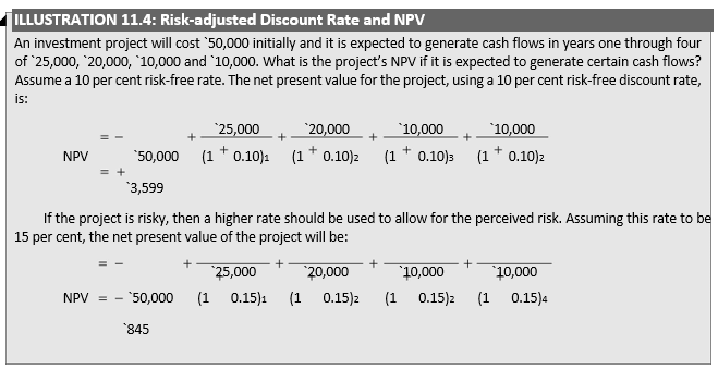
Thus, we observe that the project would be accepted when no allowance for risk is granted, but it is unacceptable if a risk premium is added to the discount rate.
In contrast to the net present value method, if a firm uses the internal rate of return method, then to allow for perceived risk of an investment project, the internal rate of return for the project should be compared with the risk-adjusted minimum required rate of return. If the internal rate of return is higher than this adjusted rate, then the project would be accepted; otherwise, it should be rejected.
Evaluation of risk-adjusted discount rate
The following are the advantages of risk-adjusted discount rate method:
It is simple and can be easily understood.
It has a great deal of intuitive appeal for risk-averse businessman. It incorporates an attitude (risk aversion) towards uncertainty.
This approach, however, suffers from the following limitations:
There is no easy way of deriving a risk-adjusted discount rate. As discussed earlier, CAPM provides for a basis of calculating the risk-adjusted discount rate. Its use has yet to pick up in practice.
It does not make any risk adjustment in the numerator for the cash flows that are forecast over the future years.
It is based on the assumption that investors are risk averse. Though it is generally true, there exists a category of risk seekers who do not demand premium for assuming risks; they are willing to pay a premium to take risks. Accordingly, the composite discount rate would be reduced, not increased, as the level of risk increases.9
Certainty Equivalent
Yet another common procedure for dealing with risk in capital budgeting is to reduce the forecasts of cash flows to some conservative levels. For example, if an investor, according to his ‘best estimate’, expects a cash flow of `60,000 next year, he will apply an intuitive correction factor and may work with `40,000 to be on the safe side. There is a certainty-equivalent cash flow. In a formal way, the certainty equivalent approach may be expressed as:

where NCFt = the forecasts of net cash flow without risk adjustment t = the risk-adjustment factor or the certainty-equivalent coefficient rf = risk-free rate assumed to be constant for all periods.
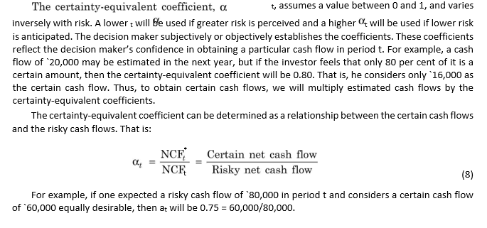
For example, if one expected a risky cash flow of `80,000 in period t and considers a certain cash flow of `60,000 equally desirable, then at will be 0.75 = 60,000/80,000.
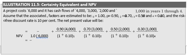
The project would be rejected as it has a negative net present value.
If the internal rate of return method is used, we will calculate that rate of discount which equates the present value of certainty-equivalent cash inflows with the present value of certainty-equivalent cash outflows. The rate so found will be compared with the minimum required risk-free rate. Project will be accepted if the internal rate is higher than the minimum rate; otherwise it will be unacceptable.
Evaluation of certainty equivalent
The certainty-equivalent approach explicitly recognizes risk, but the procedure for reducing the forecasts of cash flows is implicit and is likely to be inconsistent from one investment to another. Further, this method suffers from many dangers in a large enterprise. First, the forecaster, expecting the reduction that will be made in his forecasts, may inflate them in anticipation. This will no longer give forecasts according to ‘best estimate’. Second, if forecasts have to pass through several layers of management, the effect may be to greatly exaggerate the original forecast or to make it ultra conservative. Third, by focusing explicit attention only on the gloomy outcomes, chances are increased for passing by some good investments.
Risk-Adjusted Discount Rate vs Certainty-equivalent
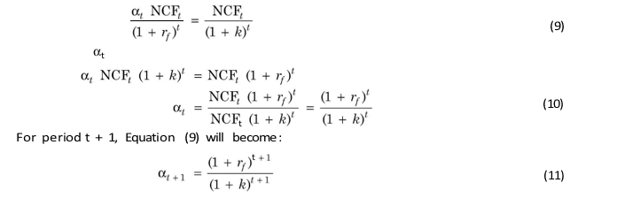
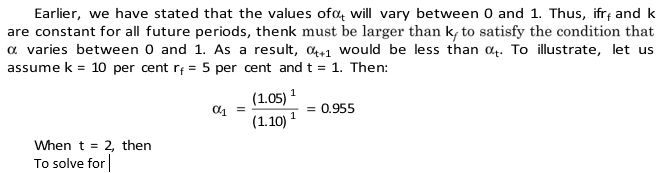
The risk-adjusted discount rate approach will yield the same result as the certainty equivalent approach if the risk-free rate is constant and the risk-adjusted discount rate is the same for all future periods. Thus,
The certainty-equivalent approach recognizes risk in capital budgeting analysis by adjusting estimated cash flows and employs risk-free rate to discount the adjusted cash flows. On the other hand, the risk-adjusted discount rate adjusts for risk by adjusting the discount rate. It has been suggested that the certainty equivalent approach is theoretically a superior technique over the risk-adjusted discount approach because it can measure risk more accurately.10
- Defend payback as a method of handling investment risk.
- What is risk-adjusted discount rate method? How does it work? What are its merits and demerits?
- What is certainty-equivalent method? How does it work? What are its merits and demerits?
- What is the difference between the risk-adjusted and the certainty-equivalent methods? Whichone is a better method of risk handling?
DECISION TREES FOR SEQUENTIAL INVESTMENT DECISIONS
We have so far discussed simple accept-or-reject decisions, which view current investments in isolation of subsequent decisions. But in practice, the present investment decisions may have implications for future investment decisions, and may affect future events and decisions. Such complex investment decisions involve a sequence of decisions over time. It is argued that ‘since present choices modify future alternatives, industrial activity cannot be reduced to a single decision and must be viewed as a sequence of decisions extending from the present time into the future.’11 If this notion of industrial activity as a sequence of decisions is accepted, we must view investment expenditures not as isolated period commitments, but as links in a chain of present and future commitments.12 An analytical technique to handle the sequential decisions is to employ decision trees.13 In this section, we shall illustrate the use of decision trees in analysing and evaluating the sequential investments.
Steps in Decision Tree Approach
At present decision depends upon future events, and the alternatives of a whole sequence of decisions in future are affected by the present decision as well as future events. Thus, the consequence of each decision is influenced by the outcome of a chance event. At the time of taking decisions, the outcome of the chance event is not known, but a probability distribution can be assigned to it. A decision tree is a graphic display of the relationship between a present decision and future events, future decisions and their consequences. The sequence of events is mapped out over time in a format similar to the branches of a tree.
While constructing and using a decision tree, some important steps should be considered:
Define investmentThe investment proposal should be defined. Marketing, production or any other department may sponsor the proposal. It may be either to enter a new market or to produce a new product.
Identify decision alternatives The decision alternatives should be clearly identified. For example, if a company is thinking of building a plant to produce a new product, it may construct a large plant, a medium-sized plant or a small plant initially and expand it later on or construct no plant. Each alternative will have different consequences. Draw a decision treeThe decision tree should be graphed indicating the decision points, chance events and other data. The relevant data such as the projected cash flows, probability distributions, the expected present value, etc., should be located on the decision tree branches.
Analyse data The results should be analysed and the best alternative should be selected.
ILLUSTRATION 11.6: Decision Tree Analysis: Water Purity Limited
Water Purity Limited has developed a scientifically more effective water filter than the ones currently available in the market. One option before the company is to start production on a large scale by installing a large plant costing `50 lakh. Alternatively, it can initially install a small plant at a cash outlay of `10 lakh and then decide to expand the capacity after a year at a cost of `45 lakh if the initial demand is high. There is a 50–50 chance that the initial demand will be high or low. If it is high, then there is a 70 per cent chance that demand in the subsequent years will be high. If it turns out to be low, it is expected to remain low in subsequent years also.
The large plant is likely to generate net cash flow of `10 lakh in year 1 if demand is high and `7 lakh if demand is low. With a high initial demand, net cash flows are expected to be `16 lakh in perpetuity if the subsequent demand is high and `10 lakh if the subsequent demand is low. The subsequent demand will remain low if the initial demand is low and the expected cash flow in perpetuity will be `7 lakh. The small plant is estimated to yield net cash flows of `4 lakh in year 1 if demand is high and `2 lakh if demand is low. If the initial demand is high, the company will expand its capacity, and it is expected to generate net cash flows of `20 lakh in perpetuity if the subsequent demand is high and `8 lakh if the subsequent demand is low. If the initial demand is low, the subsequent demand will be low, and the expected net cash flow is `2 lakh in perpetuity. What should Water Purity Limited do?
The problem of water filter in this Illustration is a sequential decision, and can be depicted as a decision tree as shown in Figure 11.1. We may notice the following in Figure 11.1:
decision points shown by squares; chance events shown by circles;
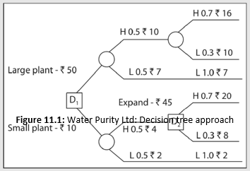
The decision points faced by the company are represented by squares. The company has to first decide whether a large plant or a small plant should be built. After one year, it has to decide whether the capacity should be expanded if the initial choice was to build a small plant. The chances of initial and subsequent demand being high and low are shown by circles, and are known as chance events. The expected net cash flows with associated probabilities are shown on the branches of tree. The probabilities of demand after year 1 depend on the demand conditions in year 1. For example, there is a 70 per cent probability that the subsequent demand will be high if demand in year 1 is high. What is the probability that demand will be high in the first year as well as the subsequent years? This is given by the joint probability of occurrences of high demand, i.e., 0.5 × 0.7 = 0.35.
In order to decide whether the company should build a large plant or a small plant, we should first analyse the problem of plant expansion after the first year. This is called the method of backward inductionor rolling back. If the initial demand is high and the company expands its plant, the expected net cash flow (ENCF) is:
ENCF = 0.7 × 20 + 0.3 × 8 = `16.4 lakh
To calculate the net present value of the expected net cash flow, we need a discount rate. Let us assume that Water Purity Limited has an opportunity cost of capital of 20 per cent. Thus the expected net present value (ENPV) of expansion costing `45 lakh at the end of year 1 is:
16.4
ENPV 45 `37 lakh
0.2
Note that ENCF of `16.4 is perpetuity, and its value is found by simply dividing it by the discount rate. What will be ENPV in year 1 if the company decides not to expand that plant? In our illustration this is possible only if the initial demand is low. The expected net cash flow will remain `2 lakh in perpetuity. Thus ENPV in year 1 is:
2
ENPV 0 `10
0.20
and ENPV today is:
2 10
ENPV 0 10
1.20
We may note that when the initial demand is low, no future decision is involved since the company will not expand. We could directly calculate ENPV as follows:
2
ENPV –10 0
0.2
since ENCF of `2 lakh is a perpetuity from the beginning.
Expansion is expected to yield a higher expected net present value if the initial demand is high. What is ENPV today if the company decides in favour of expansion? The company will have to incur an initial cost of `10 lakh. The expected net cash flow in year 1 will be `4 + `37 = `41 lakh if demand is high and `2 + `10 = `12 lakh if demand is low. Thus ENCF today is:
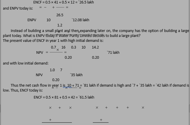
and ENPV today is:
61.5
ENPV 50 `1.25 lakh
1.2
In fact, there is no need to perform backward calculation in case of the large plant since no future decision is involved. We can calculate ENPV today as follows:
0.5 10 0.5 7 0.5[0.7 16 0.3 10] 0.5 (1 7)
ENPV = – 50 + +
1.2 0.2 (1.2)
8.5 (10.6) / 0.2 8.5 53
= – 50 + + (– 50) +
1.2 1.2
= + `1.25 lakh
Note that the expected net cash flow in perpetuity after year 1 is `10.6 lakh and its present value today is `53 lakh. Thus the expected net cash flow in year 1 is: 8.5 + 53 = `61.5 and their present value is `51.25 lakh.
Given ENPV calculations, the best alternative for Water Purity Limited seems to build a small plant today and expand it after a year if the initial demand is high. This alternative yields a higher ENPV than the other alternative.
Usefulness of Decision Tree Approach
The decision tree approach is extremely useful in handling the sequential investments. Working backwards—from future to present—we are able to eliminate unprofitable branches and determine optimum decision at various decision points. The merits of the decision tree approach are:14
Clarity It clearly brings out the implicit assumptions and calculations for all to see, question and revise.
Graphic visualizationIt allows a decision maker to visualize assumptions and alternatives in graphic form, which is usually much easier to understand than the more abstract, analytical form.
However, the decision tree diagrams can become more and more complicated as the decision maker decides to include more alternatives and more variables and to look farther and farther in time. It is complicated even further if the analysis is extended to include interdependent alternatives and variables that are dependent on one another; for example, sales volume depends on market share which depends on promotion expenses, etc. The diagram itself quickly becomes cumbersome and calculations become very time-consuming or almost impossible.
Check Your Concepts
- What are sequential investments?
- What are the steps in the decision tree analysis of sequential investments?
- What is the utility of the decision tree analysis?
| Summary | |
| Risk arises in the investment evaluation because the forecasts of cash flows can go wrong. Risk can be defined as variability of returns (NPV or IRR) of an investment project. Standard deviation is a commonly used measure of variability. Statistical techniques are used to measure and incorporate risk in capital budgeting. Two important statistics in this regard are the expected monetary value and standard deviation. The decision maker instead of working with one single forecast can work with a range of values and their associated probabilities. The expected monetary value is the weighted average of returns where probabilities of possible outcomes are used as weights. Decision makers in practice may handle risk in conventional ways. For example, they may use a shorter payback period, or use conservative forecasts of cash flows or discount net cash flows at the riskadjusted discount rates. Yet another technique of resolving risk in capital budgeting, particularly when the sequential decision making is involved, is the decision tree analysis. The decision tree provides a way to represent different possibilities so that we can be sure that the decisions we make today, take proper account of what we can do in the future. |
|
To draw a decision tree, branches from points marked with squares are used to denote different possible decisions, and branches from points marked with circles denote different possible outcomes. In a decision tree analysis, one has to work out the best decisions at the second stage before one can choose the best first stage decision.
Decision trees are valuable because they display links between today’s and tomorrow’s decisions. Further, the decision maker explicitly considers various assumptions underlying the decision. The use of decision tree is, however, limited because it can become complicated.
Review Questions
- Explain the concept of risk? How can risk be measured?
- What are the advantages of the risk-adjusted discount rate? What is the major problem in using this approach to handle risk in capital budgeting?
- What are the advantages of using the certainty-equivalent approach? Does it suffer from any limitation?
- ‘The certainty-equivalent approach is theoretically superior to the risk-adjusted discount rate.’ Do you agree? Give reasons.
- What are the limitations of payback method as a risk handling technique? Can it be used as a supplement to more sophisticated techniques?
- How can you conduct the DCF break-even analysis? Why is the DCF analysis important in risk analysis in capital budgeting?
- What is sensitivity analysis? What are its advantages and limitations?
- How can the probability theory be utilized in analyzing risk of investment projects? Illustrate.
- Describe the decision tree approach with the help of an example. How is this technique useful in capital budgeting?
- How can utility theory be incorporated in the capital budgeting decision to account for the risk preferences of the decision maker?