
8.1 Categories of investment
Before developing any theories investment choices by people it is important to define what is meant by investment.
Investment: is the formation of real capital, tangible or intangible, that will produce a stream of good and service in the future. Investment undertaken in an economy is classified according to the following categories:
1. Business fixed Investment which include plant and machinery, office buildings .
2. Residential Construction Investment which includes houses and significant additions to house ( that require building permit)
3. Changes in firm‘s Inventories –as they provide revenue in the future, not today.
4. Purchases of Durable Goods by Households for example cars, fridges.
5. Government purchases of investment Goods and Building for example roads Hospital, harbours,
6. Investment in Human Capital for example schooling university study, apprenticeships etc.
7. Knowledge which. Includes things we know about scientific and other areas.
8. The national income accounts only measure 1,2,3 and 5 as investment and it is not clears how well they measure 2 and 5 )eg. Additions not requiring permits and durables purchased by government departments|. The national accounts do not measure 6 or 7
Investment Affects Future Output
The capital is a very important used to produce output and the level of investment ultimately determines the level of the capital stock and thus the growth of output. The relationship between investment and the capital stock can be expressed in the following way:
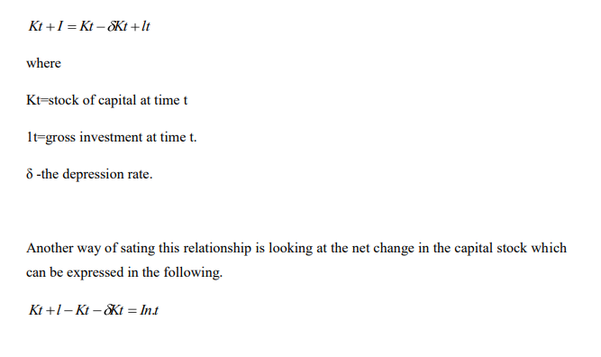
Where In,t is net investment at time t.
This implies that if . In,t increase then kt+1 increase and thus Yt+1>Yt, that is output should increase . Not that the notation used above assumes that investment undertaken today not really become productive until the future. This is usually the assumption we sue in modern macroeconomics.
Investment Fluctuates A Lot
1. A well established fact of modern economies is that 1 fluctuates a lot more C or Y ( we can also see that Y fluctuates more than C, probably because of the large fluctuations in I which helps to make up Y).
2. Furthermore, inventory investment, which makes up only a small percentage of GDP, is extremely volatile and in a recession more than half the fall in spending for a typical industrialized country comes from a decline in inventory investment as firms rundown their inventories.
As a result, if we want to explain fluctuations in output, then we need to understand what causes fluctuations in an economy‘s investment behaviors. this has been recognized for quite a long time, including by Keynes himself who put it down to ―animal spirits‖, or that fluctuations of firm‘s investments is due to seemingly random fluctuations in firm‘s expectations about future profitability, there is likely an element of truth in this view, since we have seen that people‘s consumption choices depend on future income, but it is in some sense a pessimistic view since it essentially says that investment is what it is and that is all we can say . For the rest of the lecture we shall study three categories of investment and in the process see if Keynes was right.
8.2 Business Fixed Investment
Many people are intensely interested in business fixed investment and it not difficult to understand why; it constitute the basic equipments used by firms to produce output whether it be computers, factories, machine tools or offices. We will learn about the most common theory develop to explain this form of investment.
Neoclassical theory of Investment
Our next theory of aggregate investment is the one currently used by economists. An important underlying assumption of the accelerators model is that firms do not change their production techniques In effect they employ the same proportions of capital and labour independents of their affected by output, but on the basis of cost-benefit decision. That is, firms may have a desired output level they wish to produce, given the price the output can be sold at, but the bundle of inputs they use will depend on their relative costs and benefit so as to maximize the profits of firms.
The Formal Model
We will now write the basic idea described a above as a formal model . To begin with define the following variables:
Y= the quantity of output produced by the firm
K= the quantity of capital used by the firm
L= the quantity of labour used by the firm
F(…] = the production which related how the inputs capital and labour are used to produce output.
Next, we need to specify the key assumption used by the model:
1. Firms act to maximize their profits where profits equal revenue less costs. If firms maximize profits by hiring labour and capital, then the amount they choose to hire will satisfy the condition MB = MC for each factor, or in this case their MRP equals their cost Let,
W= the marginal nominal wage paid to employees.
R= the marginal nominal ―rental‖ cost that films incur in using capital
Py= price the firms receive for their output.
P= the aggregate price level.
Where it is important to note that the implicit or explicit cost of cost of using capital is not simply the actual price of the capital, since the capital can be resold. The cost of using the using the capital is the implicit (or explicit (or explicit if rented from another firm) cost of renting the capital over the period it is used ( we will discuss this is more detail soon) which we are calling R( eg. if we build a dam and use it to produce electricity then the capital cost per unit of electricity is not the total cost of the dam, fraction of it relating to what
portion of it was use to produce the unit electricity). Given our assumption, we know that the logical implication is that capital labour are employed up to the point where.
Py x MPL= W or MPL= WPy and PY x MPK = MPK =RPy .And we will now explore more about the MB and the MC of using capital
Marginal Benefit of Using Capital
The real benefit of using capital is given by the MP that the production firms earns from the output it produces using the capital. It is also worth noting that the MP of the factors, and hence the MPK depends in general on the actual quantities of the factors used. That is, MPK = Y/ k = f [k, L]/ k
Where it is clear that the level of output depends on both L and K, in many cases economists assumes diminishing returns to the factors of production, or that as we increase the amount of a factor used output increase but at a diminishing rate. We will use this assumption here. From following the logical implications of our assumptions we have deducted that there are three things that will influence the marginal benefit of using capital:
1. Stock of capital of labour – eg the higher the stock of capital, the lower the MPK. This is just the assumption of diminishing returns to the factors of production.
2. Quantity of labour used – eg, the higher the quantity of labour used, the higher the MPK.
3. State of the production Technology- eg the better, the technology the higher the MPK.
Marginal Cost of Using Capital.
We know that the real cost of using capital is not just the capital , but is instead a fraction of this relating to the period over which the capital is used, which we have called the reakl rental cost ( or R/P bove).
This is made up of the following factors:
- Foregone Interest Earnings ( or interest costs)- say the nominal rate of interest is i then ipk is the interest cost, or the foregone interest cost, where PK is the purchase price of capital . This is fact gives you the fraction of the actual purchase price of the capital which is relevant for the period for which is used to produced things.
- Valuation losses or Gains-ie PK may go up ( valuation gains ) or go down (valuation losses) Let – ∆pk = cost of gains or loss
- Wear and tear of capital hired out- ie . the capital depreciates in values when rented out purely from its being used to produce good and services . let & = the rate of depreciation
This implies that δPK is the nominal depreciation cost
From 1-3) we now have the total cost of renting out one unit (or using) capital for producing output for one period from 1-3
Nominal cost of capital =ipk – PK+ pk = pk (i- PK/PK+ )
And to summarize, the nominal cost of capital depends on:
1. The price of capital
2. The interest rate.
3. The rate at which capital prices are changing.
4. The depreciation rate.
What we have worked out is perfectly correct, but we will invoke one more assumption to simplify the expression for the cost capital. For simplicity, assume that the price of that goods increase at the same rate the inflation rate. This can be characterized mathematically as,
PK/PK = P/P = the inflation rate
We also know that r=i-π (ie. The real interest rate is approximately equal to the nominal interest rate less the inflation rate – this should really be the expected inflation rate, but how do we get real cost of capital = Pk/p(r + )
This tells us that we can expect that real cost of capital to depend upon
1. The relative price of the capital good
2. The real interest rate
3. The depreciation rate
PROFIT Rate of capital
Now we know that the determine both the MB and the MC of using and thus owing capital we are now in a position to answer the basic question of how mush capital should firms in total use and own. The answer to this is that it all depends on the profit rate of capital, which equal, profit rate =revenue –cost= MPk- (pk/p)r+δ)
There are three cases to consider.
1. MPK> cost of capital means there are potential profits a firms could earn by increasing its capital stock k and the amount of net investment is positive (ie. Kt+1>Kt).
2. MPK < cost of capital means the firms is making losses on the last units of capital it is using and it could increase profits by reducing its capital stock k and the amount of net investment is negative (ie kt+1<kt)
3. MPK = cost of capital means the firms is maximizing the amount of profit it can earn from using capital and does not want to change its to capital stock , or reduce it through depreciation depends upon the profit rate or the different between the MPK and the cost of capital. Note that unlike the accelerators theory shows us what determines that optimal or desired capital stock , it is the amount of capital where MB= MC , or no more profit can be made from changing firm‘s amount of capital
8.3 Investment and the Capital Stock
A Logical conclusion from the neoclassical theory of investment is that both net gross investment of firms are a negative function of r because the cost of capital is positively affected by changes in r which negatively affected the profit rate of capital we can show this relationship graphically as:
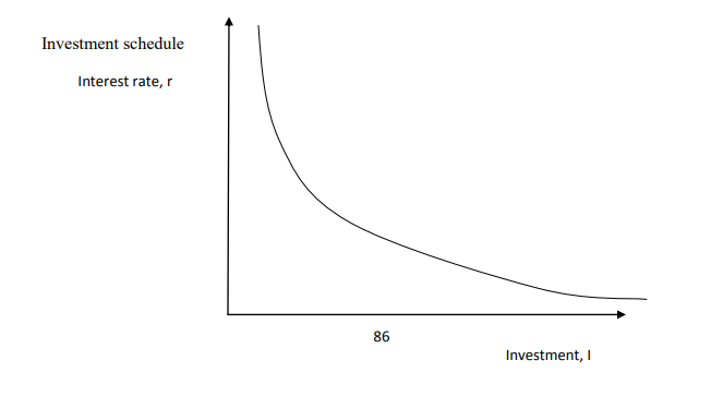
And a change in any other variable that affected by MB or MC OF using and owing capital MPK , say from a technological innovation, cause a rightward shift in the investment schedule. The amount of investment that is undertaken depends on whether or not firms are using and owning the optimal amount of capital amount of capital, that is , whether or not the profit rate is zero or non-zero. In the long run equilibrium, with the profit rate we would expect that the amount of the net investment is zero with gross investment being positive and just offsetting the amount of depreciated capital each period. Once a firm is in its long – run state only a change in R or MPK, or some other variable, will cause net investment demand. This will cause net investment to stop being zero and the capital stock will adjust to get back to a new long – run equilibrium situation
Effects of Tax Laws
We have focused on a few key variables which affect the amount of investment undertaken but in reality anything which affects the cost or benefit or using capital will affect the amount government taxes let r be the tax rate on firms‘ revenues. Then the after tax profit rate of capital equal , profit rate =(1 –r ) Mpk –(PK/P)( r+δ) so that we can see that the tax reduces the profits earned from capital by reducing the MB of using and owing capital. For example, three common policies which affect investment are.
1. Taxes on income earned from owing capital.
This is simply the company tax isn‘t directly levied on capital income but on a company‘s profits, which include income and cost from all factors, but some proportion of its incidence is on income earned from capital and we can think of it this way . An increase in the company tax will effectively increase r and hence decrease i . This sort of policy will discourage the accumulations,
2. Investments tax credits
This is a policy where firms ‗tax liabilities are reduced by how much they spend on new capital during a year .This effectively lowers r reducing the cost of capital and causing and increase in I. This sort of policy will encourage the accumulation of K
Tax Treatment of Department Depreciation
Corporate profits are taxed and profits are just revenue minus costs. Part of the Cost of production of firms is depreciation on capital so that firms are allowed to Include depreciation of their capital as a cost when calculating the amount of Profit to be taxed but depreciation of their capital as a cost when calculating the a amount of profit to be taxed but depreciation the true cost of depreciation in period of high inflation which overstate the profits being made this means a tax is levied even if the economic profit is Zero , which effectively increase r reducing I and discouraging the accumulation of capital . The third type of policy is a factor because obviously the IRD to say something about the treatment of depreciation for firms that have to file tax returns.
8.4 Residential Investment.
Another type of investment dear to the hearts and wallets of many Kenyans, as wall as involving large expenditures, and one which varies strongly with the business cycle, is residential investment what we want to know is that factors determine investment in residences and how they do so.
8.4.1 Neoclassical Model of Residential Investment
The neoclassical model of residential investment directly uses an important conceptual thinking about capital. : the existing capital and investment but is made explicit in the mode learn about . The idea I s that there are two part to the housing market ; the mark existing stock of house which determine the equilibriums housing prices and the new housing which determine the flow of residential investment . Note that this is a new housing which determines the flow of investment. Note that this is a for all forms of capital but we are using it explicitly here in our model,
8.4.2 The formal model
First off, define the following variables:
PH= the going price of housing in an economy.
P= the price going of housing in economy.
KH= stock of residential capital or housing
IH=investment in housing.
Determining the equilibrium price PH/P- the market for Existing house as normal market the relative price of housing PH/P is determined jointly by den supply. The stock of houses is fixed in the short tern and so the supply curve of houses is vertical. If we invoke the assumption of the law of demand then the housing is of the Norman downward sloping from in the relative price of
housing. Given a fixed population the demand for housing can change if the relative pricing of housing change. It is easy to see why using example. Say for example PH/P then the quantity demanded falls because.
- People live in small house
- People share residences
- Homelessness
8.4.3 Determining investment –the supply of new housing
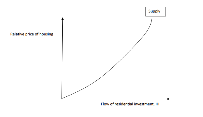
We know that the supply that of housing does change does over time . we also know that the costs of building new houses is made of up of materials, hiring labour and hiring capital ( tools , machines etc).these form the MC of building new housing. We will assume the law of supply that extra quantities of new housing is more expensive because of diminishing returns to the factors of production used by the firms. That is , the existing resources become more expensive as firms bid up their prices to get them ; additional factors requires higher payment s to induce them to supply their services, or the additional factors are just as existing resources used. The
MB for firms or developer from building new housing is the relative price of housing. to induce construction firms to build new house the MB , or relative price o housing has to higher than the MC this tells us that supply of new housing curve sloping in the relative price of new housing .The supply of new housing can be characterized graphically as follows:
Changes in he Demand for and supply Housing
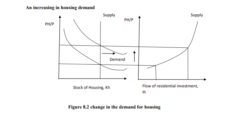
We now have formal model of the residential housing. Any change in the relative price of housing curves movement a long the existing curves as per normal supply and demand curves any other change involves a shift of a curve which will have other flow on effects. We look at one particular example. Say a country‘s population increase either because of an increase in the reproduction because of higher net immigration. this causes the following sequence of things to 1
1) Demand for housing curve shifts outwards
2) PH/P to clear the housing market.
3) Supply of a new housing increase, increasing the future stock of housing this cause a fall in PH/P although it will still be higher than the original level.
The change in the demand for housing can be characterized graphically as follows:
There are many other things that can affected the demand for housing rate ( ie because it affects mortgage costs, or the opportunity cost of holding housing )‘ the tax deductibility of interest payment ( ie if these exist they increase from owing house better technology , expecially in builing materials and techniques as it lowers the cost of supply new houses and thus shifts the supply down incomes of people ( ie how much income people have affect their damand and host of other factors.
Summary
1) Demand for housing increases when the population increase (immigration are better of( higher real gdp) per capital growth)
2) Prices act to ration out scarce resources.
3) We never really get to an ―equilibrium‖, in the static meaning of equilibrium, because shocks are always occurring! but our economic reasoning tells us what effects the shocks will have and in which direction economic variables will change in response to them.
8.5 Inventory investment
The last category of investment that we will study is inventory investment. It is not that large compared to the other forms of investment, but as mentioned at the beginning of this topic there is a strong relationship between changes in inventory investment and changes in output over the business cycle.
8.5.1 Reasons for holding inventories
Before developing a theory of inventory investment we will study the reasons why inventories are held. Knowing the reasons for holding inventories will help us understand better the factors which influence the level of inventory investment. There are four reasons for holding inventories:
1) Production smoothing: often it is cheaper to produce goods at a steady rate, than to continually alter production runs. This means that during slow periods inventories build up and during boom periods inventories are run down.
2) Inventories as a factor of production: films carry inventories of spare parts incase a machine breaks down, so that the entire assembly line does not come to a stop. E.g. car assembly factory.
3) Stock out avoidance: to avoid lost sales and profits when sales may be unexpectedly high e.g. a book retailer may carry multiple copies of a book if they are not sure how popular the book will be.
4) Work in process: partly completed productions are counted as inventories e.g. cheese making where cheeses are aging.
An important point to notice about all of these reasons is that have a short-term focus and not a long-term focus as with the other forms of investment. This suggests that they will not be so heavily influenced buy short-run changes in relative prices but will instead be tied closely to output. Another point to note is that reason 1.is not likely to be an important reason why inventories fluctuate during business since this sort of inventory investment goes up as output goes down whereas inventory investment as a whole goes down as output goes down. This means 2.-4 must be the main cause of fluctuations in inventory investment during a business cycle.