We discuss the consumption choices of individuals .the theory of intertemporal choice was developed by irving fisher (1867-1947)the intertemporal choice theory is about individual not aggregate consumption but it does not have important implication for aggregate consumption because aggregate consumption is the sum of consumption by individuals fisher observed that people do not just have a budget constraint for today or for the current period but also for tomorrow or the future .he further observed that people can trade off consumption today for consumption tomorrow by saving or not saving. This means that the budget constraints for each period are linked together. The collection of budget constraint for all the periods plus the linkages between them gives us the inter-temporal budget constraints. This is the constraint limiting the choices; people have between consuming today and consuming tomorrow
YC=current received by consumers
Yf=future income received by consumers
Cc=current consumption of the consumers
Cf=future consumption
S=how much the currently save
R=interest rate R>0.
If people prefer consuming today rather than in the future This implies that the budget constraint today can be written as Cc=Yc-S Or the level of consumption today equals the level of income less what was saved.
If borrowing occurs, then s is <0 so, current consumption is greater than current income S<0 and Cc>Yc The budget constraint in the future is given by Cf=(1+r)s+Yf Or the level of consumption in the future +future income +whatever has been saved from today.
if S>0, then there is positive interest positive interest as well as future Y.if S>0,then the consumer pays some of their income to repay the borrowing that occurred today at the interest rate incurred S+Yc-Cc
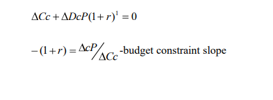
Substituting the equation tomorrow‘s budget constraint Cf+(1=r)(Yc-Cc)+Yf…………………2 Rearranging this equation and dividing both sides by (1+r) we get the following equation Cc+Cf(1+r) 1 =Yc+Yf(1+r) 1 …………………………intertemporal budget constraint
It is important to note that if r>0, then future income and consumption are discounted. This discounting of future income and consumption occurs because of the interest earned on savings The discount factor(1+r) is the price of the future consumption measured in terms of today‘s consumption .it is the amount of current consumption that the consumer I must give up to obtain one unit of future consumption .Since r>0,then (1+r)1 is a unit of current consumption If borrowing or saving did not take place then the budget constraint would just be Yc=Cc and future budget constraint will be Yf=Cf
7.2 Consumer preference
Fischer observed that people will have preferences regarding consumption over different periods .we represent such preferences in the following diagram
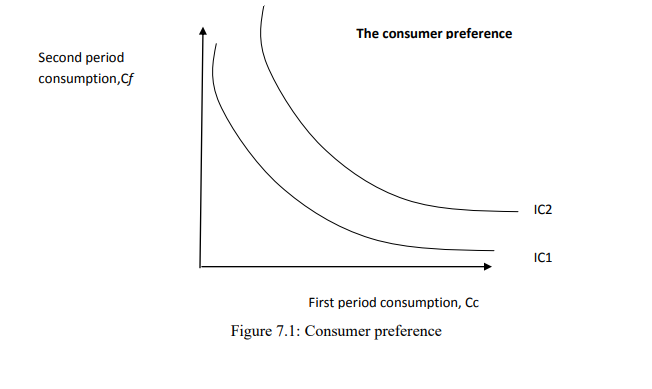
The indifference curve shows the combination of current and future consumption that makes the consumer equally happy. The slope at any point on an indifference curve measures the MRS between current and future consumption. Higher Indifference curves are preferred to lower indifference curve
7.3 Optimal consumption point
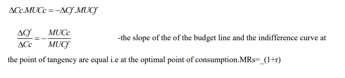
Assume that consumers chose their consumption to maximize their utility. Given the income of the consumer and the interest rate, the consumer will therefore choose the highest indifference curve that their budget constraint allows. This occurs where the budget line is target to indifference curve
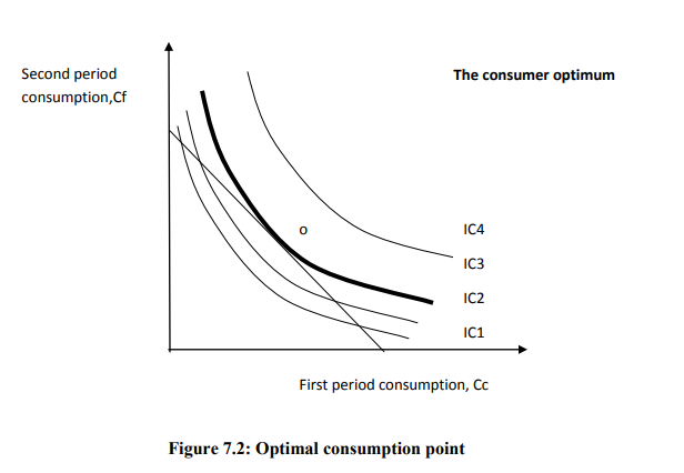
It is important to note that there is a key characteristic of this point of tangency .it occurs where the slope of the budget line we =slope of the indifference curve. A long the budget line, any substitution s between current and future substitution must offset each other
A long the indifference curve, the utility a person gets is the same ,this means that any substitution on the indifference curve between the current and future period consumption must offset each other
Factors Affecting Consumption
7.4.1 Effect of changes in income on consumption
Say the current of future income increases. A change in income either today or in the future has the same effect; it increases a person’s present value income. That is it increases, yc+yf(1+r).we show this by a shift outwards in the budget line
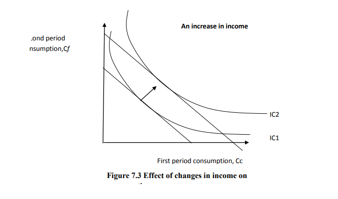
If Cc and Cf are both normal goods then their consumption increases. That is, the consumer spreads the increase in income over both current and future consumption regardless of when the income increases. This tells us that current consumption primarily depends on the present value over income over the life time of a person not just on current income. Current income does not affect current consumption because it affects the present value of lifetime income, but is only a small part of it and so changes in current income will have only a small effect on current consumption. Not that this can occur because the consumer will have only small effects on current consumption. Note that this can occur because the consumer is free to borrow and lend as much as they wish at the going interest rate subject to their not going bankrupt
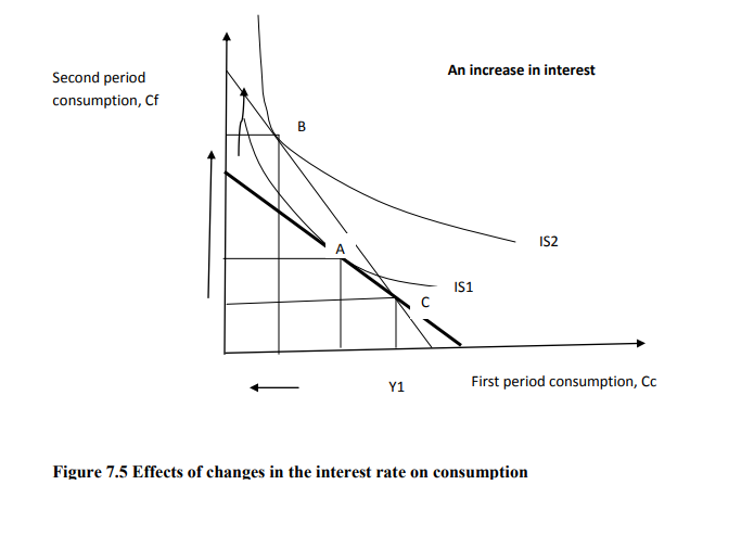
7.4.2 Effects of changes in the interest rate on consumption
An obvious variable that is part of the intertemporal budget constraint is the interest rate .it determines the price for trading off consumption between periods and the value to saving or the cost of borrowing. When we think about an individual and a change in the interest rate we have to consider two cases
- When the consumer borrows ,or is a dissever(s,0)
- When the consumer lends or is a saver(s>0)
There are two effects arising from increase in interest rates
- Income effect –this is the change in consumption resulting from the movement to a different indifference curve. Given that the consumer is a lender, rather tan a borrower they are better off and end up on a higher indifference curve in period 1.income effect implies increases in cc and increases in cf
- Substitution effect-refers to a change in consumption resulting from the change in relative price of consumption in two periods. Given that r has increased then current consumption is relatively more expensive compared to future consumption? Substitution effect implies a fall in cc and an increase in cf. Overall .we know that cf increases but we cannot say for certain what happens to cc. The end result depends on which effect is stronger the graph www.masomomsingi.com 73 shows that the case where substitution effect dominates the income effect. Note that we are assuming that Cc and Cf are normal goods when analyzing the income effect
7.4.3 Effects of changes in wealth on consumption
A common item which s thought to affect people‘s consumption is people‘s wealth. In Newzealand and Australia it is commonly claimed that when people‘s houses increase in value then this leads to an increase in their consumption. Similarly for increases in the value of shares in the US. How can we think about this when the intertemporal budget constraint does not contain a wealth variable? Easy .wealth, or our stock of assets, simply increases the present value of resources we have available to spend on consumption. That is, if we are considering not just income but all our resources then we just add our stock of assets to the income we earn to get the true present value lifetime resources. Say we denote the present value of our assets as a, then our present value lifetime resource constraint is Yc+yf(1+r+a)
This means that a y change in the value of our assets or wealth will have the same impact on our consumption as a change in our income. if the value of our assets increases ,the present value of lifetime resources increases, which is shown by a rightward parallel shift of the budget constraint and if consumption is a normal good ,then we will consume more both today b and in future. Note that to make it simpler, we can just think conceptually of future income including both income earned and also the value our assts which could be sold (this reduces the number of symbols without changing our results)
7.5 Theories of Aggregate Consumption
1) Absolute Income Hypothesis/Keynesian consumption function
This theory of aggregate consumption was derived by john myriad Keynes in 1930s.Keyne made some three main assumptions
- 0<MPC< where MPC=DC/DY or the MPC is the amount of extra consumption out of etra dollar of income
- APC increases as Y increases where APC =C/Y ar the APC is the ratio of total consumption total income
- Y is the predominant determinant of C and r has little impact on C. Given these three assumptions ,the Absolute income hypothesis can be written as
Ct=C+cYt where C>0 and 0<c<1
Ct—is aggregate consumption
C-is called autonomous consumption
c-is the marginal propensity to consume
Yt-is aggregate disposable income
This model captures the KCF or the AIH because
- The MPC ,c ,is between 0 and 1by assumption
- The interest rate is assumed to have no effect on aggregate consumption and this is shown by by its being not included in the aggregate consumption function
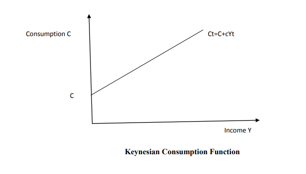
- The APC falls as income increases which we can show by rearranging our model;APC=CtYt=CYt+c which tells us that as Yt increases then Cyt also decreases. the following graph shows what the KCF looks like and low it relates to consumption
Keynesian Consumption Function
The success of any theory and model is that they are consistent with the relevant to the real world data. What about the KCF/AIH? Sometimes after Keynes theory was developed, households were surveyed and it was found out that
- Richer households consumed more than poor ones. MPC>0
- Richer households saved more than poor ones .MPC<1
- Richer households saved larger fractions of their income which means that APC increases as Yt increases Consumption C Income Y C Ct=C+cYt Keynesian Consumption Function
- The correlation between income and consumption was found to be very strong .so this on this evidence the KCF seemed to be consistent with the available real world data about consumption
The consumption puzzle Unfortunately for Keynes and his KCf, during the 1940s two pieces were produced that were not consistent with the KCF predictions about how aggregate consumption and savings should behave
SECULAR STAGNATION DID NOT OCCUR
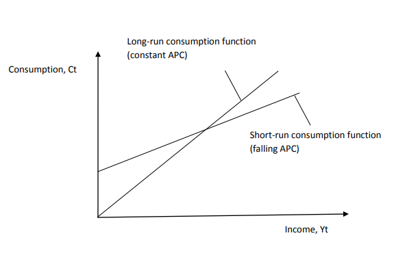
The first anomaly had to do with a theoretical implication of the KCF that as Y increases, C increases but proportionately less than income. This means the pool of savings increases more than proportionately as income rose. Since savings equals investment in equilibrium, investment increases proportionately more than income. But the problem is that it does not make sense for firms to want to keep m, investing if people were buying proportionately smaller levels of consumption goods as compared to their incomes A long differential of infinite duration commonly referred to as circular stagnation would then occur. It was thought that once the 2nd world war ended, thus ending the large government demand for goods and services that the economy will enter a period of secular stagnation .But, it did not! What actually happened conflicted with the theory of Keynes about how aggregate consumption depended on aggregate income The KCF was not consistent with new time series data After Keynes developed the KCF, Simon Kuznets created data from the US national accounts from 1869 to the 1940s on aggregate Y and C. It showed that C was very stable fraction of Y even as Y increased a lot. This conflicted with the KCF .The difference arose between this study and the earlier ones that supported the KCF because the early studies were cross-sectional in detail(they looked at a snapshot of the economy at a point)whereas Kuznets study was o a time series nature(It looked at the economy over many points in time)So the evidence seemed to indicate that there were two consumption functions: a short-run consumption function in which the APC was basically constant with different levels of Y. This an be graphically shown as below
2)The Life Cycle hypothesis
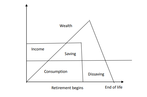
The KCF while able to explain aggregate consumption of the economy at a point in time was able to explain it over time. This led to the new ways of trying to explain aggregate consumption. Two theories were developed at about the same time .i) one theory was developed by Franco Modigliani ,Alberto Ando and Richard Brumberg.in the 1950s.They argued that it is not only income in the current period that affected people‘s observed consumption choices but also income they expected in the future. they hypothesized that the income of the people varies in a known way over people‘s ;lives and that people use savings to move income from high income periods to low income periods known now as the life cycle hypothesis. it is the application of the fisher model
LIFE CYCLE PROFILE