INVENTORY MANAGEMENT NOTES

INTRODUCTION

Inventories constitute the most significant part of current assets for a large majority of companies in India. On an average, inventories are approximately 60 per cent of current assets in public limited companies in India. Because of the large size of inventories maintained by firms, a considerable amount of funds is required to be committed to them. It is, therefore, absolutely imperative to manage inventories efficiently and effectively, in order to avoid unnecessary investment. A firm neglecting the management of inventories will be jeopardizing its long-run profitability and may fail ultimately. It is possible for a company to reduce its levels of inventories to a considerable degree, e.g., 10 to 20 per cent, without any adverse effect on production and sales, by using simple inventory planning and control techniques. The reduction in ‘excessive’ inventories carries a favourable impact on a company’s profitability.

NATURE OF INVENTORIES

Inventories are stock of the product a company is manufacturing for sale and components that make up the product. The various forms in which inventories exist in a manufacturing company are: raw materials, work-in-process and finished goods.

Raw materials are those basic inputs that are converted into finished product through the manufacturing process. Raw material inventories are those units which have been purchased and stored for future productions.

Work-in-process inventories are semi-manufactured products. They represent products that need more work before they become finished products for sale.

The levels of three kinds of inventories for a firm depend on the nature of its business. A manufacturing firm will have substantially high levels of all three kinds of inventories, while a retail or wholesale firm will have a very high level of finished goods inventories and no raw material and work-in-process inventories. Within manufacturing firms, there will be differences. Large heavy engineering companies produce long production cycle products; therefore, they carry large inventories. On the other hand, inventories of a consumer product company will not be large because of short production cycle and fast turnover.
Finished goods inventories are those completely manufactured products which are ready for sale. Stocks of raw materials and work-in-process facilitate production, while stock of finished goods is required for smooth marketing operations. Thus, inventories serve as a link between the production and consumption of goods.

Firms also maintain a fourth kind of inventory, supplies or stores and spares. Supplies include office and plant maintenance materials, like soap, brooms, oil, fuel, light bulbs, etc. These materials do not directly enter production, but are necessary for production process. Usually, these supplies are small part of the total inventory and do not involve significant investment. Therefore, a sophisticated system of inventory control may not be maintained for them.

NEED TO HOLD INVENTORIES

The question of managing inventories arises only when the company holds inventories. Maintaining inventories involves tying up of the company’s funds and incurrence of storage and handling costs. If it is expensive to maintain inventories, why do companies hold inventories? There are three general motives for holding inventories.¹

Transactions motive, which emphasizes the need to maintain inventories to facilitate smooth production and sales operations.

Precautionary motive, which necessitates holding of inventories to guard against the risk of unpredictable changes in demand and supply forces and other factors.

Speculative motive, which influences the decision to increase or reduce inventory levels to take advantage of price fluctuations.

A company should maintain adequate stock of materials for a continuous supply to the factory for an uninterrupted production. It is not possible for a company to procure raw materials whenever it is needed. A time lag exists between demand for materials and its supply. Also, there exists uncertainty in procuring raw materials in time, on many occasions. The procurement of materials may be delayed because of factors such as strike, transport disruption or short supply. Therefore, the firm should maintain sufficient stock of raw materials at a given time to streamline production. Other factors which may necessitate purchasing and holding of raw material inventories are quantity discounts and anticipated price increase. The firm may purchase large quantities of raw materials than needed for the desired production and sales levels to obtain quantity discounts of bulk purchasing. At times, the firm would like to accumulate raw materials in anticipation of a price rise.

Work-in-process inventory builds up because of the production cycle. Production cycle is the time span between introduction of raw material into production and emergence of finished product at the completion of production cycle. Till the production cycle completes, stock of work-in-process has to be maintained. Efficient firms constantly try to make production cycle smaller by improving their production techniques.

Check Your Concepts
Stock of finished goods has to be held because production and sales are not instantaneous. A firm cannot produce immediately when customers demand goods. Therefore, to supply finished goods on a regular basis, their stock has to be maintained. Stock of finished goods has also to be maintained for sudden demands from customers. In case the firm’s sales are seasonal in nature, substantial finished goods inventories should be kept to meet the peak demand. Failure to supply products to customers, when demanded, would mean loss of the firm’s sales to competitors. The level of finished goods inventories would depend upon the coordination between sales and production as well as on production time.

1. What is the nature of inventories? What is included in inventories?
2. What are the reasons for holding inventory?
3. Explain transaction, precautionary and speculative motives for holding inventories.

OBJECTIVE OF INVENTORY MANAGEMENT

In the context of inventory management, the firm is faced with the problem of meeting two conflicting needs:

To maintain a large size of inventories of raw material and work-in-process for efficient and smooth production and of finished goods for uninterrupted sales operations. To maintain a minimum investment in inventories to maximize profitability.

Both excessive and inadequate inventories are not desirable. These are two danger points within which the firm should avoid. The objective of inventory management should be to determine and maintain optimum level of inventory investment. The optimum level of inventory will lie between the two danger points of excessive and inadequate inventories.

The firm should always avoid a situation of over investment or under-investment in inventories. The major dangers of over investment are: (a) unnecessary tie-up of the firm’s

 

funds and loss of profit, (b) excessive carrying costs, and (c) risk of liquidity. The excessive level of inventories consumes funds of the firm, which then cannot be used for any other purpose, and thus, it involves an opportunity cost. The carrying costs, such as the costs of storage, handling, insurance, recording and inspection, also increase in proportion to the volume of inventory. These costs will impair the firm’s profitability further. Excessive inventories, carried for long-period, increase chances of loss of liquidity. It may not be possible to sell inventories in time and at full value. Raw materials are generally difficult to sell as the holding period increases. There are exceptional circumstances where it may pay to the company to hold stocks of raw materials. This is possible under conditions of inflation and scarcity. Work-in-process is far more difficult to sell. Similarly, difficulties may be faced to dispose off finished goods inventories as time lengthens. The downward shifts in market and the seasonal factors may cause finished goods to be sold at low prices. Another danger of carrying excessive inventory is the physical deterioration of inventories while in storage. In case of certain goods or raw materials deterioration occurs with the passage of time, or it may be due to mishandling and improper storage facilities. These factors are within the control of management; unnecessary investment in inventories can, thus, be cut down.

Maintaining an inadequate level of inventories is also dangerous. The consequences of under-investment in inventories are: (a) production hold-ups and (b) failure to meet delivery commitments. Inadequate raw materials and work-in-process inventories will result in frequent production interruptions. Similarly, if finished goods inventories are not sufficient to meet the demand of customers regularly, they may shift to competitors, which will amount to a permanent loss to the firm.

ensure a continuous supply of raw materials, to facilitate uninterrupted production. maintain sufficient stocks of raw materials in periods of short supply and anticipate price changes.
The aim of inventory management, thus, should be to avoid excessive and inadequate levels of inventories and to maintain sufficient inventory for the smooth production and sales operations. Efforts should be made to place an order at the right time with the right source to acquire the right quantity at the right price and quality. An effective inventory management should:

maintain sufficient finished goods inventory for smooth sales operation, and efficient customer service. minimize the carrying cost and time. control investment in inventories and keep it at an optimum level.

Check Your Concepts

1. What are the two conflicting needs of inventory management?
2. What are the objectives of effective management of inventory?

INVENTORY MANAGEMENT TECHNIQUES

In managing inventories, the firm’s objective should be in consonance with the shareholder wealth maximization principle. To achieve this, the firm should determine the optimum level of inventory. Efficiently controlled inventories make the firm flexible. Inefficient inventory control results in unbalanced inventory and inflexibility—the firm may sometimes run out of stock and sometimes may pile up unnecessary stocks. This increases the level of investment and makes the firm unprofitable.

To manage inventories efficiency, answers should be sought to the following two questions:

How much should be ordered? When should it be ordered?

The first question, how much to order, relates to the problem of determining economic order quantity (EOQ), and is answered with an analysis of costs of maintaining certain level of inventories. The second question, when to order, arises because of uncertainty and is a problem of determining the reorder point.²

Economic Order Quantity (EOQ)

One of the major inventory management problems to be resolved is how much inventory should be added when inventory is replenished. If the firm is buying raw materials, it has to decide the lots in which it has to be purchased on replenishment. If the firm is planning a production run, the issue is how much production to schedule (or how much to make). These problems are called order quantity problems, and the task of the firm is to determine the optimum or economic order quantity (or economic lot size). Determining an optimum inventory level involves two types of costs: (a) ordering costs and (b) carrying costs. The economic order quantity is that inventory level that minimizes the total of ordering and carrying costs.

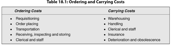
Ordering Costs

Carrying Costs
The term ordering costs is used in case of raw materials (or supplies) and includes the entire costs of acquiring raw materials. They include costs incurred in the following activities: requisitioning, purchase ordering, transporting, receiving, inspecting and storing (store placement). Ordering costs increase in proportion to the number of orders placed. The clerical and staff costs, however, do not have to vary in proportion to the number of orders placed, and one view is that so long as they are committed costs, they need not be reckoned in computing the ordering cost. Alternatively, it may be argued that as the number of orders increases, the clerical and staff costs tend to increase. If the number of orders are drastically reduced, the idle clerical and staff force can be used in other departments. Thus, these costs may be included in the ordering costs. It is more appropriate to include clerical and staff costs on a pro rata basis. Ordering costs increase with the number of orders; thus the more frequently inventory is acquired, the higher the firm’s ordering costs. On the other hand, if the firm maintains large inventory levels, there will be few orders placed and ordering costs will be relatively small. Thus, ordering costs decrease with increasing size of inventory.

Costs incurred for maintaining a given level of inventory are called carrying costs. They include storage, insurance, taxes, deterioration and obsolescence. The storage costs comprise cost of storage space (warehousing cost), stores handling costs and clerical and staff service costs (administrative costs), incurred in recording and providing special facilities, such as fencing, lines, racks, etc. Table 18.1 provides summary of ordering and carrying costs.

Carrying costs vary with inventory size. This behaviour is contrary to that of ordering costs which decline with increase in inventory size. The economic size of inventory would thus depend on trade-off between carrying costs and ordering costs.

Ordering and Carrying Costs Trade-off

The optimum inventory size is commonly referred to as economic order quantity. It is that order size at which annual total costs of ordering and holding are the minimum. We can follow three approaches—the trial and error approach, the formula approach and the graphic approach—to determine the economic order quantity (EOQ). We assume that total annual demand is known with certainty and usage of materials is steady. Also, ordering cost per order and carrying cost per unit are assumed to be constant.

Trial and Error Approach

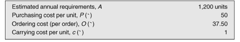
The trial and error, or analytical, approach to resolve the order quantity problem can be illustrated with the help of a simple example. Let us assume the following data for a firm:

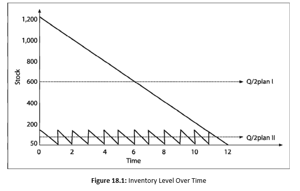
If we assume annual requirements as known and steady usage, the inventory levels under different lot size alternatives are shown in Figure 18.1. For illustrative purposes, we have depicted only two alternatives—placing one order in the beginning or 12 monthly orders. The single order plan (say, Plan I) involves an average inventory level of 600 units, starting with the highest level of 1,200 units and ending with zero level. On the other hand, the multiple order plan entailing 12 orders results in an average inventory level of 50 units.
A number of alternatives are available to the firm. It may purchase its entire requirement of 1,200 units in the beginning of the year, in one single lot or in 12 monthly lots of 100 units each and so on. If only one order of 1,200 units is placed, the firm will have a starting inventory of 1,200 units. With the constant consumption, the inventory size will reduce in a systematic way and will reach zero level at the end of the year. As the firm will hold 1,200 units in the beginning and zero unit at the end of the year, the average inventory held during the year will be 600 units, [i.e., (1200 + 0)/2 = 600 units], representing an average value of `30,000 (600 × `50). On the other hand, if the monthly purchases are made, 12 orders of 100 units each will be placed during the year. Thus, the firm will have 100 units at the start of a month and zero unit at the end of the month and the average inventory held will be 50 units (i.e., (100 + 0)/2 = 50 units), representing an average value of `2,500 (50 × `50). Many other possibilities can be worked out in the same manner. If the objective is to minimize the inventory investment, then monthly orders or even less than that, if possible, may be favoured. However, this may not be most economical. To determine the economical order size, implications of both carrying and order costs should be studied.³

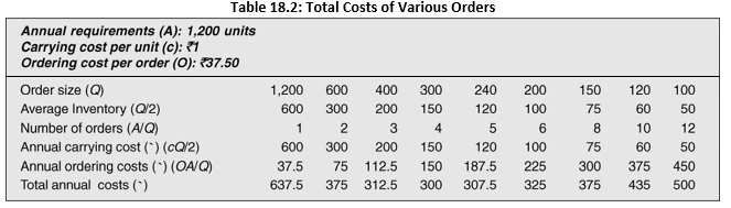
The multiple order plan (say, Plan II) involves less investment in inventories; but it is not necessarily the most economic plan. To determine optimum order quantity, a comparison of total costs at different lot sizes should be made. The computations are shown in Table 18.2.

In terms of the total annual costs, Plan II is preferable, as it has a total annual cost of `500 as against the total annual cost of `637.5 of Plan I. But for an economic solution, other alternatives should also be considered. Computations in Table 18.2 show that the total annual cost is minimum, i.e., `300 when the number of orders in the year is 4. The economic order quantity, therefore, is 300 units.

Order-formula Approach

The trial and error, or analytical, approach is somewhat tedious to calculate the EOQ. An easy way to determine EOQ is to use the order-formula approach. Let us illustrate this approach.⁴

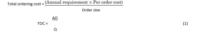
Suppose the ordering cost per order, O, is fixed. The total order costs will be number of orders during the year multiplied by ordering cost per order. If A represents total annual requirements and Q the order size, the number of orders will be A/Q and total order costs will be:

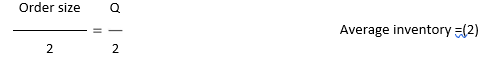
Let us further assume that carrying cost per unit, c, is constant. The total carrying costs will be the product of the average inventory units and the carrying cost per unit. If Q is the order size and usage is assumed to be steady, the average inventory will be:

and total carrying costs will be:

Total carrying cost = Average inventory × Per unit carrying cost

Qc

TCC =(3)

The total inventory cost, then, is the sum of total carrying and ordering costs: Total cost = Total carrying cost + Total order cost

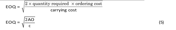
Equation (4) reveals that for a large order quantity, Q, the carrying cost will increase, but the ordering costs will decrease. On the other hand, the carrying costs will be lower and ordering cost will be higher with the lower order quantity. Thus, the total cost function represents a trade-off between the carrying costs and ordering costs for determining the EOQ. Economic order quantity is calculated as follows:

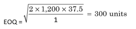
To illustrate the use of EOQ formula, let us assume data of the example, taken to illustrate the trial and error approach. As assumed earlier, if the total requirement is 1,200 units, ordering cost per order is `37.50 and carrying cost per unit is `1, the economic order quantity will be:
We note from Equation (5) that EOQ changes directly with total requirements, A, and order cost O, and has an inverse relationship with the carrying cost, c. However, the squareroot sign restrains the relationship in both cases. Thus, if the usage is double, the economic order quantity is not doubled; it will increase by, or about 1.4 times.⁵

This corresponds with the answer found out by trial and error approach.

Graphic Approach

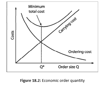
The economic order quantity can also be found out graphically. Figure 18.2 illustrates the EOQ function. In the figure, costs—carrying, ordering and total—are plotted on vertical axis and horizontal axis is used to represent the order size. We note that total carrying costs increase as the order size increases, because, on an average, a larger inventory level will be maintained, and ordering costs decline with increase in order size because a larger order size means less number of orders. The behaviour of total costs line is noticeable since it is a sum of two types of costs which behave differently with order size. The total costs decline in the first instance, but they start rising when the decrease in average ordering cost is more than offset by the increase in carrying costs.⁶ The economic order quantity occurs at the point Q* where the total cost is minimum. Thus, the firm’s operating profit is maximized at point Q*.

It should be noted that the total costs of inventory are fairly insensitive to moderate changes in order size. It may, therefore, be appropriate to say that there is an economic order range, not

a point. To determine this range, the order size may be changed by some percentage and the impact on total costs may be studied. If the total costs do not change very significantly, the firm can change EOQ within the range without any loss.⁷

Reorder Point

The problem, how much to order, is solved by determining the economic order quantity, yet the answer should be sought to the second problem, when to order. This is a problem of determining the reorder point. The reorder point is that inventory level at which an order should be placed to replenish the inventory. To determine the reorder point under certainty, we should know: (a) lead time, (b) average usage, and (c) economic order quantity. Lead time is the time normally taken in replenishing inventory after the order has been placed. By certainty, we mean that usage and lead time do not fluctuate. Under such a situation, reorder point is simply that inventory level which will be maintained for consumption during the lead time. That is:

Reorder point = Lead × Average usage                                                                               (11)

Safety Stock
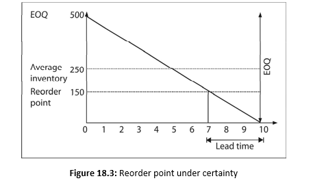
To illustrate, let us assume that the economic order quantity is 500 units, lead time is three weeks and average usage is 50 units per week. If there is no lead time, that is, delivery of inventory is instantaneous, the new order will be placed at the end of tenth week, as soon as EOQ reaches zero level. But, if the lead time is three weeks, the new order should be placed at the end of seventh week, when there are 150 units left to consume during the lead time. As soon as the lead time ends and inventory level reaches zero, the new stock of 500 units will arrive. Thus, the reorder point is 150 units (50 units × 3 weeks). This is illustrated in Figure 18.3. which shows that the order will be placed at the end of seventh week, where 150 units are left for consumption during the lead time. At the end of tenth week, the firm will get a supply of 500 units. If the lead time is nil, the re-order point will be the zero level of inventory.

In our example, the reorder point was computed under the assumption of certainty. It is difficult to predict usage and lead time accurately. The demand for material may fluctuate from day-today or from week-to-week. Similarly, the actual delivery time may be different from the normal lead time. If the actual usage increases or the delivery of inventory is delayed, the firm can face a problem of stock-out which can prove to be costly for the firm. Therefore, in order to guard against the stock-out, the firm may maintain a safety-stock—some minimum or buffer inventory as cushion against expected increased usage and/or delay in delivery time. Assume in the previous

example, the reasonable expected stock-out is 25 units per week. The firm should maintain a safety stock of 75 units (25 units × 3 weeks). Thus, the reorder point will be 150 units + 75 units = 225 units. The maximum inventory will be equal to the economic order quantity plus the safety stock, i.e., 500 units + 75 units = 575 units. Thus, the formula to determine the reorder point when safety stock is maintained is as follows:

Reorder point = Lead × Average usage + Safety stock                                                          (12)

Large numbers of firms have to maintain several types of inventories. It is not desirable to keep the same degree of control on all the items. The firm should pay maximum attention to those items whose value is the highest. The firm should, therefore, classify inventories to identify which items should receive the most effort in controlling. The firm should be selective in its approach to control investment in various types of inventories. This analytical approach is called the ABC analysis and tends to measure the significance of each item of inventories in terms of its value. The high-value items are classified as ‘A items’ and would be under the tightest control. ‘C items’ represent relatively least value and would be under simple control. ‘B items’ fall in between these two categories and require reasonable attention of management. The ABC analysis concentrates on important items and is also known as control by importance and exception (CIE).⁸ As the items are classified in the importance of their relative value, this approach is also known as proportional value analysis (PVA).
Figure 18.3 shows the reorder point under the assumption of the safety stock.

The following steps are involved in implementing the ABC analysis:

Classify the items of inventories, determining the expected use in units and the price per unit for each item.

Determine the total value of each item by multiplying the expected units by its units price.

Rank the items in accordance with the total value, giving first rank to the item with highest total value and so on.

Compute the ratios (percentage) of number of units of each item to total units of all items and the ratio of total value of each item to total value of all items.

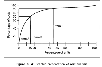
Combine items on the basis of their relative value to form three categories—A, B and C. The data in Table 18.3 and Figure 18.4 illustrate the ABC analysis.

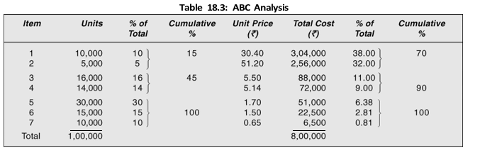
The tabular and graphic presentation indicate that ‘Item A’ forms a minimum proportion, 15 per cent of total units of all items, but represents the highest value, 70 per cent. On the other hand, ‘Item C’ represents 55 per cent of the total units and only 10 per cent of the total value. ‘Item B’ occupies the middle place. Items A and B jointly represent 45 per cent of the total units and 90 per cent of the investment. More than half of the total units are ‘Item C’, representing merely 10 per cent of the investment. Thus, a tightest control should be exercised on ‘Item A’ in order to maximize profitability on its investment. In case of ‘Item C’, simple controls will be sufficient.

Summary

Inventories constitute about 60 per cent of current assets of public limited companies in India. The manufacturing companies hold inventories in the form of raw materials, work­in­process and finished goods. There are at least three motives for holding inventories.

To facilitate smooth production and sales operation (transaction motive).

To guard against the risk of unpredictable changes in usage rate and delivery time (precautionary motive). To take advantage of price fluctuations (speculative motive).

Inventories represent investment of a firm’s funds. The objective of the inventory management should be the maximization of the value of the firm. The firm should therefore consider: (a) costs, (b) return, and (c) risk factors in establishing its inventory policy.

Two types of costs are involved in the inventory maintenance:

Ordering costs: requisition, placing of order, transportation, receiving, inspecting and storing and clerical and staff services. Ordering costs are fixed per order. Therefore, they decline as the order size increases. Carrying costs: warehousing, handling, clerical and staff services, insurance and taxes. Carrying costs vary with inventory holding. As order size increases, average inventory holding increases and therefore, the carrying costs increase.

The firm should minimize the total cost (ordering plus carrying). The economic order quantity (EOQ) of inventory will occur at a point where the total cost is minimum. The following formula can be used to determine EOQ:

where A is the annual requirement, O is the per order cost, and c is the per unit carrying cost.

The economic order level of inventory, Q^*, represents maximum operating profit, but it is not optimum inventory policy. The value of the firm will be maximized when the marginal rate of return of investment in inventory is equal to the marginal cost of funds. The marginal rate of return (r) is calculated by dividing the incremental operating profit by the incremental investment in inventories, and the cost of funds is the required rate of return of suppliers of funds.

When should the firm place an order to replenish inventory? The inventory level at which the firm places order to replenish inventory is called the reorder point. It depends on (a) the lead time and (b) the usage rate. Under perfect certainty about the usage rate, and instantaneous delivery (i.e., zero lead time), the reorder point will be equal to: Lead time × usage rate.

In practice, there is uncertainty about the lead time and/or usage rate. Therefore, firms maintain safety stock which serves as a buffer or cushion to meet contingencies. In that case, the reorder point will be equal to: Lead time × Usage rate + Safety stock. The firm should strike a trade­off between the marginal rate of return and marginal cost of funds to determine the level of safety stock.

A firm, which carries a number of items in inventory that differ in value, can follow a selective control system. A selective control system, such as the A­B­C analysis, classifies inventories into three categories according to the value of items: A­category consists of highest value items, B­category consists of high value items and C­category consists of lowest value items. More categories of inventories can also be created. Tight control may be applied for high­value items and relatively loose control for low­value items.

Review Questions

1. Why should inventory be held? Why is inventory management important? Explain the objectives ofinventory management?
2. ‘There are two dangerous situations that management should usually avoid in controlling inventories.’Identify the danger points and Explain.
3. Define the economic order quantity. How is it computed?

• ‘The practical approach in determining economic order quantity is concerned with locating a minimumcost range rather than a minimum cost point.’ Explain.
  ‘The management of inventory must meet two opposing needs.’ What are they? How is a balance broughtin these two opposing needs?

5. What are ordering and carrying costs? What is their role in inventory control?
6. Define safety stock? How can safety stock be computed?
7. What are the cost of stock-outs? How should the costs of stock-out and the carrying costs be balanced toobtain the optimum safety stock?
8. How is the reorder point determined? Illustrate with an example and graphically.
9. What is lead time? How does it affect the computation of reorder point under certainty and uncertainty?
10. What is a selective control of inventory? Why is it needed? Illustrate with an example and graph theABC analysis.
11. Explain the steps involved in analysing investment in inventories? Illustrate with an example.

Quiz Exercises

1. A firm’s cost of carrying one unit of inventory is `5. The cost per order of inventory is `2,000. The firm’s annual usage of inventory is 1,00,000 units. What is the firm’s EOQ?
2. A company has `6 per year carrying cost on each unit of inventory, an annual usage of 1,20,000 units and an ordering cost of `200 per order. Calculate the economic order quantity. If a quantity discount of `0.25 per unit is offered to the company when it purchases in lots of 1,000 units, should the discount be accepted?
3. A manufacturing company has an expected usage of 5,00,000 units of certain product during the nextyear. The cost of processing an order is `100 and the carrying cost per unit is `2 for one year. Lead time on an order is five days and the company will keep a reserve supply of three days’ usage. You are required to calculate (a) the economic order quantity and (b) the reorder point. (Assume 360-day year).
4. A firm’s estimated demand for a material during the next year is 25,000 units. Acquisition costs are`250 per order and carrying cost is `5 per unit. The safety stock is set at 25 per cent of the EOQ. The daily usage is 100 units and lead time is 10 days. Determine (a) the EOQ, (b) the safety stock, and (c) the reorder point. (Assume 250-day working in a year).