
Examples of linear equations in economics
There are several types or examples of linear equations as used in Economics.
The main examples are:
- The production possibility frontier; a graph that shows combinations of goods and services that can be produced with a given level of resources.
- The demand function; an equation showing the various quantities of goods purchased by customers at given prices.
- The supply function; an equation showing the various quantities of goods brought to the market by suppliers at a given market price.
- Isocost line; a graph showing different combinations of labour and capital that can be purchased by a given firm.
The demand curveTHE DEMAND CURVE
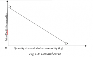
The demand curve shows the relationship between the quantity demanded of a commodity and the price of that commodity. This is a negative slope. It shows that an increase in the independent variable (price) leads to a decrease in the dependent variable (quantity demanded).
The supply curve
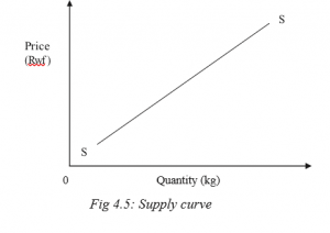
The supply curve shows the relationship between the quantity supplied of a commodity to the market by suppliers and the price of the commodity. This has a positive slope. It shows that both the price (the independent variable) and quantity supplied (the dependent variable) change in the same direction.
4.1.2 Non linear equations and non linear graphs
Non-linear algebraic equations are polynomial equations of a degree that is greater than one. They are mathematical relationships that describe non linear graphs. They take various types. For instance, we have the following main non- linear equations:
- Polynomials
- Logarithmic equations
- Conic equations
- Exponetioal equation
1 Necessary conditions for simultaneous equations
These conditions include that:
- There should be more than one functional relationship, between a set of specified variables such as x and y or q and p.
- That all the functional relationships are in linear form. It is then that we try to find the value of the unknown variables in the equations. In the case where we have only two variables in the equations, it is then possible to subject the equations to graphical solutions.
Simultaneous equations can be solved using various methods.
4.1.3.2 Methods used in solving simultaneous equations
- a) The substitution method
This method entails representing one unknown in terms of the other unknown
Other examples of non linear graphs in Economics a) Average cost curve
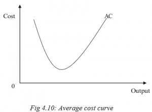
The average cost curve (AC) shows the relationship between the output produced and the variable cost spent on producing each unit of this output.
- b) The average product curve
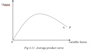
The average product curve (AP) shows the relationship between the variable factor employed and the output produced from each unit of the variable factor.
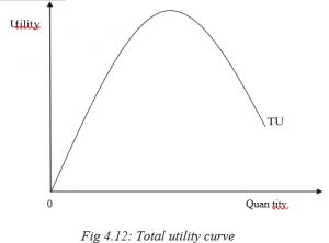
- c) Total utility curve
A differential equation is a mathematical equation that relates some function with its derivatives. Functions are usually represented by physical quantities. Derivatives represent the rates at which the physical quantities change. Thus differential equations define the relationship between the two.
Differential equations have types. For instance:
- Ordinary differential equations.
- Partial differential equations.
An ordinary differential equation (ODE) is an equation that contain a function of one independent variable and its derivative
Linear and non-linear differential equations
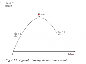
Maxima and minima points
Maximum (maxima) and minimum (minima) points have an important application
Percentage is a way of expressing the magnitude of a given quantity in relation to 100 such quantities. It shows the amount, number or rate of something as part of a total of 100.
In the case of the firm of Simon in Activity 4.7 given at the beginning of this unit, we saw that the ratio of the dairy cattle being milked to the total number of dairy cattle was 4:5 or 4/5. This is because, out of the total 50 dairy cattle, 40 were being milked. To find the percentage of these cattle being milked to the total number, we would divide 40 by 50 and then multiply by 100 for example 40 or 40/50 then multiply the result by 100. This would give us a figure of 80. We would then say that 80 percent of the dairy cattle on the farm are being milked. This is written as 80%.
This concept of percentages is of great significance in economic analysis. This is because it gives a quick glimpse of the magnitude of a given variable in relation to a total. For example, if we are told that the youth of country X constitute 60% of the total population of that country, this gives us an immediate and clear idea of the magnitude of the population problem.
At the work place, it would also be more meaningful to talk of the number of female employees in percentage terms as a way of determining the extent of equity in employment. It is also more meaningful to the common person when changes in certain economic parameters are expressed in terms of percentages rather than in absolute terms. We are therefore more comfortable when told of a 10% increase in the cost of living or a 20% increase in the level of wages.
In microeconomics, percentage is mainly used to determine the degree of changes in:
- Price
- Quantity
- Elasticity
- Costs
- Profit
In macroeconomics, calculation of percentages is mainly done to determine macroeconomic indicators like:
- Gross domestic growth (GDP)
- Inflation rates
- Unemployment rates
Reciprocals
The reciprocal of a number would be given by dividing 1 by that number. For example, the reciprocal of 4 would be 1/4. In the case of fractions, the reciprocal would be derived by inverting the fraction. Thus the reciprocal of 2/5 would be 5/2.
The concept of reciprocals is widely applied in economic analysis. For example, it is used in the calculation of the multiplier in banking and investment decisions. In such a case, the multiplier is determined by calculating the reciprocal of the marginal propensity to save. This is based on the assumption that people’s income is spent on either consumption or saving. The proportion of the income that would be spent on saving is what would be referred to as the marginal propensity to save.
Averages
When loosely stated, the average refers to the centre of a series of data. It is one of what is commonly referred to as measures of central tendency. It is found by adding the values of the data provided and then dividing by the total number of values. For example, if we are given the weekly sales of a shopkeeper as follows:
| Monday | Tuesday | Wednesday | Thursday | Friday | Saturday |
| $90 | $120 | $80 | $60 | $60 | $150 |
Then the average sales for the shopkeeper would be: $103.3.
(Obtained by adding the daily sales, then dividing the sum by six, the number of days).
We would then say that the average daily sales for the shopkeeper is $103.3.
This concept is used in various ways as an aid to decision making. It could
be used to determine the average level of wages earned by a given group of workers, or to determine the average sales made by a team of salespersons. In Economics, the concept of the average is very important. For example, economists use the concept in analysing investment and production decisions. They will therefore talk about the average cost of production which is the total production divided by the number of units produced, as opposed to the average revenue which is the total revenue divided by the number of units sold. Comparison of the two averages can indicate the direction in which a business is going.
Index numbers in Economics are usually used to establish changes in the cost of living of the people. They are usually constructed to show the difference in the price of a commodity from one period to another. In constructing such index numbers, we select one year which we belief to have been relatively stable, and call it the base year. We give this year an index value of 100. For example, if the price of sugar in 2010 was $1.00 while in 2014 it rose to $1.2, then the price would have risen in the period by 40%.
If we take 2010 to be the base year, then the index value for 2014 would be 140. The figure 140, which relates the two prices for the two years, is called the price relative. If this was true for a wide range of commodities, then we could assert that the cost of living has risen by 40% between 2010 and 2014.
To determine such change in the cost of living, we construct what is called a consumers cost of living index. In this case, we consider a range of commonly used consumer products and get their relative price changes in the period under review. We then get the average of this price changes so as to determine an overall change in the cost of living.
In Economics, index numbers are used in prices of commodities to arrive at simple price index, especially to determine the consumer price index. They are also used to determine the rate of human development to derive human development index.
4.2.6 Absolute values
In making calculations, it is usual to come up with a figure that has either a plus or a minus sign. However, such a sign may not be of any importance for making the desired decision. What may be important is the magnitude of the number without any consideration of the sign. We would therefore ignore the sign. This is the idea behind the concept of absolute numbers. The absolute number is the actual number without any consideration of the sign. Thus if we have the absolute number would be 3. Same case for a sign.
In Economics, when we talk about elasticity of demand, the coefficient of elasticity could be either positive or negative. However, for decision-making purposes, it is the absolute number that is considered.