Further Aspects of Markets and Prices; Factor Markets

MARKET STRUCTURES AND ECONOMIC WELFARE

In Study Unit 7 we examined the main forms of market structure – perfect competition, monopolistic competition, oligopoly and monopoly.  At the start of our examination we noted that it has long been a common belief among many economists that the structure of a market influences the conduct of firms operating in it and that this conduct in turn influences their performances.  The main areas of conduct likely to be affected by the competitive conditions of the market are those of:

• price setting
• advertising and marketing
• attitudes to innovation and investment – quality standards – customer care.

Conduct in these areas is likely to affect the firm’s performance in relation to profit and the efficiency with which it uses scarce resources.

Elements of Economic Welfare

By ‘economic welfare’ we mean the use of scarce resources to bring the greatest benefit to the largest possible number of people in the community.  Welfare is said to be maximised when resources are used and production distributed in such a way that it is impossible to make one person better off without making another person worse off.

Achievement of a high level of welfare clearly requires the efficient use of resources and it is usual to identify two kinds of efficiency – technical or production efficiency and allocative efficiency.

• Production or technical efficiency arises when producers are able to increase the quantity of goods and services from a given quantity of production factors. This kind of efficiency can be measured without too much difficulty.  For example, we can calculate how many motor cars one firm can produce from a set quantity of capital and labour and compare this figure with the number of similar vehicles produced from the same amount of capital and labour by a rival producer.
• Allocative efficiency relates to the distribution of production to meet the expressed wants of the community. It is of no great benefit to the community to become more technically efficient in the production of motor cars if there is already a surplus of these but a severe shortage of other goods, say homes to live in.  A production system would achieve allocative efficiency if it were able to eliminate both surpluses and shortages.  The measurement and achievement of allocative efficiency presents rather more problems than technical efficiency given the basic economic problem of unlimited wants and scarce resources.  If there are never going to be enough resources to satisfy everyone there will always be some who feel that there are not enough of certain goods or services and others who consider that resources could be better used on the forms of production they consider to be of most importance.

The greatest difficulties in determining allocative priorities are usually experienced in the public sector, where the relationship between receiving the utility or benefit of a service is separated from paying the price (meeting the factor costs) of providing that service.  Arguments about the relative importance of, say, providing more nursery education as opposed to extending care for the elderly, tend to assume that the costs of both will be paid by some third group, usually anonymous or simply referred to as “the taxpayer” or “the government”.  In this way pressure groups desiring more of their own favoured benefit avoid the difficult matter of opportunity cost.

The difficulties still exist in the market economy, or the private sector of the mixed economy, but they become focused on the question of willingness and ability to pay for the options available.

In an earlier study unit we suggested that a consumer’s marginal utility for a good would be equal to the price that consumer was willing to pay for the good.  If we accept this then the good’s market demand curve can be regarded as the aggregate of all the marginal utilities of the consumers willing to pay any price for the good.  Each point on the curve represents the utility of the marginal buyer at that point – the buyer who is prepared to pay that price but not a higher price.  A lower price brings in additional buyers whose marginal utilities are now equal to that reduced price.  Looked at in this way the market demand curve becomes a marginal social valuation curve – i.e. the value to the marginal user at each level of production.

On the supply side of the market the marginal cost curve represents the cost of producing each additional unit of the good.  This cost depends on the prices of the inputs in the factor markets and these factor prices are influenced by the community’s valuation of other possible uses for the same factors.  We may thus see the marginal cost curve as the community’s marginal social cost curve.

This view of market demand and supply is illustrated in Figure 8.1, where we see that if production of this particular good rises above q_o its marginal social cost is greater than its value to the community.  If production is lower the community would gain from increased production because its marginal value is higher than its marginal social cost.  Only at the production level q_o are these social costs and values equal.

The implication for achieving allocative efficiency is that the prices for goods should just equal their marginal costs.  If the whole production system could be organised in such a way that market prices for all goods and services were just equal to their marginal costs the community could be achieving the highest possible level of allocative efficiency.

This kind of argument is the basis for the belief expressed in many economics textbooks that the equality of price and marginal cost is an ideal to be pursued in the interests of increasing efficiency and raising the level of economic welfare.  However, it ignores a number of important issues, in particular:

• Those goods which are clearly valued by society but which are not paid for directly by their immediate users. These include the examples of education and care of the elderly.

Few very young children have incomes of their own and relatively few of the elderly in need of care have incomes able to meet the marginal costs of its provision.

• Income inequalities that exist in most market economies. As a result of these inequalities we cannot really guarantee that all market demand curves are true representations of the marginal social valuation curves of many goods on which the community as a whole is likely to place a high value.  Housing is an issue which presents difficulties for many societies.  An economic system which produces massive inequalities in housing provision cannot really claim to have achieved a high level of allocative efficiency whatever the relationship between house market prices and marginal costs.

 

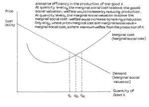
Figure 8.1:

  Allocative Efficiency in the Production of the Good X Competitive Markets and Economic Welfare

One of the problems that economists have sought to solve is the question of which type of market is most likely to increase production and allocative efficiency and, therefore, raise the level of economic welfare.

In traditional microeconomics perfect competition has often been favoured on the grounds that in the so-called long run equilibrium for the firm under perfect competition the following desirable objectives are achieved:

• Abnormal profit is eliminated
• Price is equal to marginal cost
• Firms are obliged to produce at quantity levels where average costs are at their lowest.

However, it is possible to raise a number of serious objections to this view of perfect competition.

• Long-run equilibrium can only be achieved if demand remains constant over a reasonably long period. If demand fluctuates, as it frequently does in competitive markets, the market is extremely unstable.  Firms face constantly fluctuating prices and have to plan production under conditions of considerable uncertainty.  This leads to instability in factor (including labour) prices.
• Market instability and low profit levels make it difficult to undertake technical research. Consequently firms tend to remain small and the level of technology low.  Although firms may be forced to minimise production costs these may be at levels significantly higher than could be achieved if they were able to gain economies of large-scale production and develop more advanced production technology.  Resources are not, therefore, used to their maximum potential efficiency.
• As pointed out earlier, goods that are homogeneous offer no choice to consumers and choice is an element in consumer utility.

If, then, there are doubts about the real efficiency of perfect competition, how do the other market structures compare?

Monopolistic competition does offer choice but it suffers from most of the potential defects of perfect competition.  Monopoly offers potential gains from economies of scale, the avoidance of resource duplication when competing firms produce similar goods and try to sell to the same customers, and profits are available for technical development.  However, the absence of competition removes many of the pressures that force managers to be efficient and profits may be distributed to senior managers and shareholders rather than used for research and development.  Monopoly power can lead to less rather than more efficiency in all its aspects.

Oligopoly is usually classed with monopoly in its effects on efficiency and oligopolists are often accused of collusive behaviour in order to create partial monopolies for their own benefit.  There have been many examples of collusive behaviour and abuse of market power but some modern studies have shown that apparent oligopolies can sometimes be highly competitive and the possibilities for potential compensation can produce some of the benefits of competition with less wasteful duplication of resources.

Clearly there are no simple solutions to the problems of increasing efficiency.

   PRICE DISCRIMINATION

So far, all our discussions of equilibrium and market price have assumed that suppliers will charge the same price to all consumers at any one time-period within any given supply range.  Thus, if the market price is RWF5 per kilo, this will be the price paid by Mr A Van Rooyen and by the Gold Plate Corporation.  Suppliers do not discriminate between customers but charge all the same price.

However, in practice, there is often price discrimination between buyers.  Economists have identified the following three types of price discrimination.

First Degree Discrimination

This is the most extreme form.  Suppliers seek to charge each individual customer a price equal to his marginal utility, i.e. they will try to charge the highest price that each customer is prepared to pay.  This is often called “haggling”.  Private houses (other than new houses) and second-hand cars are usually sold in this way.  In many countries, most goods are sold by haggling – a practice which has also been termed “perfect price discrimination”.  If successful, such total price discrimination will achieve the highest possible revenue – as is illustrated in Figure 8.2.

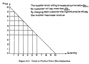
Figure 8.2:  Total or Perfect Price Discrimination

This, of course, is a seller’s ideal which is almost impossible to achieve.  Moreover, there are costs involved.  Haggling is time-consuming and possible only when there are relatively few customers in relation to the time available for selling.  When the number of customers rises, the cost of haggling exceeds the extra revenue gained, and sellers usually move towards a fixed-price system – especially when unskilled assistants have to be employed.  Haggling is profitable only when the seller is more skilled than the buyer!  There is also the danger that those who paid RWF8 will meet those who paid RWF4, feel cheated and refuse to buy any more.  Some degree of monopoly power is desirable for successful long-term, total price discrimination.

Second Degree Discrimination

This is the term sometimes applied where a selected number of large customers are charged prices lower than could be justified on the grounds of any large-scale economies achieved.  If a customer buys in bulk, then some price reduction is normal because the unit costs of selling, administration and transport are all likely to be lower.  It is not price discrimination when such cost savings are shared with the customer.  Nor is it price discrimination when customers are given incentives to adopt cost-cutting practices, e.g. to pay quickly before being sent accounts, or as soon as accounts are submitted; to order regularly, thus saving selling expenses; or to take orders at times and in quantities suited to the sellers’ needs.

Price discrimination implies a price reduction to particular customers, made simply to obtain an order that would not otherwise be given, or to encourage loyalty from a customer whom the seller would not wish to lose.

A case of second degree price discrimination is illustrated in Figure 8.3.  Notice here that the average revenue does not match any price actually charged to any customer.  Again, there is the danger that customers paying the higher price will learn of the practice and become alienated towards the supplier.  Some degree of monopoly power is, clearly, desirable from the seller’s point of view.  There is also a danger that the low-price buyer will re-sell to other customers at an intermediate price, though monopoly power would make this practice short lived.

 

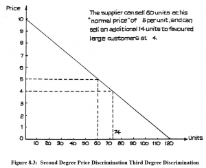
Figure 8.3:  Second Degree Price Discrimination Third Degree Discrimination

This is the term used to describe the situation where two or more separate markets can be identified and segregated.  This is illustrated in Figures 8.4 and 8.5.

Here, there are two separate markets.  Market A is made up of customers willing to pay up to RWF16 per unit.  Market B customers will pay only up to RWF10.  In this particular case, the maximum market size in each is the same, at 500 units.  At all prices, we see that demand is more price elastic in market B than in A.  The curve in B is less steep, indicating that customers are more price conscious and demand reacts more to any change in price.

The curve for the combined market is the addition of A and B.  At prices above RWF10 it reflects A’s curve only, but at lower prices it is the sum of the two separate curves.

We can adapt Figure 8.4 to show how the firm can gain from price discrimination.  Figure 8.5 adds a marginal cost curve and marginal revenue curves to the diagram.  If the firm charges the same price in both markets and does not discriminate, then its profit-maximising price, where marginal revenue = marginal cost, is RWF8.  At this price, total sales are 350 units, and total revenue is RWF8 × 350 = RWF2,800.

 

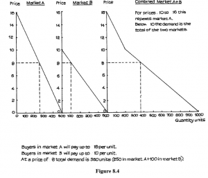
Figure 8.4

Suppose the firm can charge different prices in each market without any alteration in costs.  The marginal cost remains unchanged, and this is indicated by the horizontal MC line just below 4 on the vertical axis.  If it charges profit-maximising prices in each market, it will seek to equate this marginal cost with the marginal revenue (MR) in each of the markets A and B.  This produces a price in A of RWF9.60, at which price 200 units are sold, and a price of RWF7 in market B with sales in B of 150 units.

Total quantity sold remains unchanged at 350 units.  50 units are lost in A but 50 are gained in B.  Total revenue, however, rises to RWF2,970, made up of 200 units at RWF9.60 plus 150 units at RWF7.  Because costs remain unchanged, the additional revenue must mean that profits rise.  Notice that the rise in price in market A, where demand is more inelastic, is greater than the fall in price in market B, so that the revenue gained from the practice of discrimination is greater than the amount of revenue lost.

We can say, then, that, in order to gain from price discrimination in two different markets, price elasticity of demand at the relevant price range must be different.  At the same time, price discrimination can be operated successfully only if the two markets can be kept completely separate.  Sometimes, small differences may be made, to make it appear that the two markets are different – e.g. the difference between first- and second-class rail travel.  This represents price discrimination if the difference in fares is greater than any cost difference caused by the difference in service, standard of comfort, etc. (normally, it is).  There are also similar class differences in air travel.  Services markets are often easier to separate than goods – largely because they cannot be stored and re-sold.

Monopoly power is not necessary for price discrimination in services, though it helps if all suppliers adopt similar practices, which then gain public acceptability more easily.

 

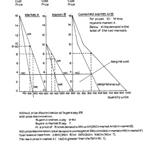
Figure 8.5

Using Spare Capacity

A rather different practice which is sometimes described as price discrimination is that of making use of spare capacity at a price which covers variable costs and makes some contribution to fixed costs.  Thus, a manufacturer may accept an order below his normal price, if his machines and labour would otherwise not be fully used.  Any price will increase profit, provided it is more than the marginal costs of meeting the order, and does not lead to pressure for reduced prices from other customers.

In the same way, a coach service may offer cheaper fares on scheduled services on certain days of the week, when otherwise coaches would be running with many empty seats.  The “standby” air fare, whereby the airline offers a low price in order to fill a seat which would otherwise remain empty is based on the same principle.  However, if these measures become too popular, they defeat their purpose.  Demand is simply transferred from one time-period to another, rather than increased, and total revenue is reduced.  It is often found, therefore, that such special price arrangements can be offered only for limited periods; otherwise all prices are reduced and profits transformed into losses.

The object of any form of price discrimination is to increase revenue more than any increase in cost that may be incurred.  Price discrimination which increases quantity demanded without any increase in profit is a failure.  A reduction in quantity supplied or a change in the pattern of demand without change in total quantity supplied could also be justified if this resulted in a reduction in costs greater than any reduction in revenue.  However, price discrimination normally leads to some increase in cost so that a greater increase in revenue would normally be needed for the practice to result in a profit rise.

 FACTOR MARKETS

In order to produce any goods or services, the business organisation has to acquire production factors.  We have already seen that the payments made to production factors make up the costs of the business.  The price that has to be paid to obtain factors forms the costs of production.  We must now examine some aspects of how factor prices are determined.

Determining Factor Prices

Just as the products of business organisations are sold in markets at prices which, subject to any market imperfections, are the result of the interaction of the forces of supply and demand, so also are the production factors.

There are factor markets, just as there are product markets – only, in factor markets the business organisations are the buyers, and they provide the demand.  The sellers are the factor owners, e.g. the owners of land or capital and people who supply their own labour.  In cases where trade unions have a very high degree of control over the people who may work in an occupation and the terms and conditions under which they may be employed, the union could be considered to be the supplier, and a number of economic models are based on this assumption.

The factor markets, therefore, are those for land, finance for capital investment and labour.  The markets for basic natural resources, such as metals, and the basic commodities required for production or for foods, are also normally regarded as being very close to factor markets.  The factor, land, is often seen as including the resources of the land which are required for production to take place.

Most of the structural features used to classify markets as described earlier, i.e. perfect competition, monopoly, etc., can also be applied to factor markets.  At the same time, however, there are some special features which apply to factor markets, and we need to take these into account.

Professionalism

The buyers and sellers of factors tend to be more expert than consumers, especially in distinguishing differences in quality.  In the consumer field, it is possible to create differences in essentially identical articles by branding, pricing, and advertising, so that buyers can be persuaded to pay more for certain goods in the belief that they are buying superior quality.  In the factor markets, this still takes place but to a lesser extent.  In markets for basic materials, careful systems of grading usually apply as for example on the London Metal Exchange for Tin ore cassiterite.

The actual buying and selling tends to become a specialised function in a factor market, so that the broker or skilled agent is important.  Tin is bought and sold in the London Metal Exchange by brokers who have to be members of specialist associations.  The skilled agent operating as a consultant has not gained an important place in the labour market, but is beginning to be more common in the field of management selection.

Alternative Uses of Factors

Factors are simply means to an end – the desired end being the production of consumer or capital goods, or the giving of a service.  As it is the end which is important, rather than the means, there will usually be a variety of ways in which factors can be combined in order to produce a particular final product (the “production function”).  In a market operating through the price system, the aim is to find the cheapest combination which will produce a given level and quality of output.

Firms which wish to achieve this combination will be influenced by changes in factor prices and by new inventions.

 Changes in Factor Prices

If copper becomes more expensive, it might be possible to use aluminium as a substitute.  If labour becomes more expensive because of pay rises or employment taxes, more extensive use may be made of capital in the form of labour-saving machinery.  If land is very expensive, a firm may use a computer and highly-skilled staff to control stocks, so that less land is devoted to the storage of material.  Capital and labour will thus replace land if their total additional cost is lower than that of the land saved.

 Inventions

New discoveries change the production function.  We are familiar with the developments which have helped to replace manual labour by capital in the form of earth-moving equipment, office machinery, computers, and electronically-controlled factory machines.  In addition, modern developments in transport and communications, the building of new roads, and the extension of electric and gas power has given firms greater freedom in the choice of location, so that there is now a greater amount of land available for industrial use.  The principle of substitution is not new but it is the key to the understanding of factor markets.

Supply of Factors

Factors of production are supplied in return for money incomes – wages, salaries, rent, fees, profits and interest are all incomes to factors.  As a general rule, we can say that more will be supplied at a higher price (assuming that people wish to maximise their incomes).

Although supply will tend to increase in response to a price rise, this may not happen immediately.  It may be very difficult, or even impossible, to increase supply in the very short run.  The supply for skilled labour, in particular, is often very inelastic in the short run, so that, in a complex industrial economy where the time element is of great importance to employers, an increase in demand may produce a steep rise in wages.

The supply of factors to particular markets should be distinguished from the supply of factors to all markets, i.e. to the economy as a whole.  Total supply may be unchanged but the distribution of supply may vary as conditions in particular markets become more – or less – favourable to the owners of the factors.

The total supply of factors to the economy as a whole is governed by rather different considerations.

 Supply of Land

For most countries, land, of course, is fixed in supply with only relatively small increases possible from reclaiming land from the sea, mountains or jungle, and in some cases this can have environmental consequences of serious concern for the future.  The productivity of land in some countries can be improved with irrigation and its industrial-commercial potentialities transformed with improved communications.

Supply of Capital

Capital is a more mobile factor; huge amounts of it are moved around the world by the large multinational companies.  The total quantity of productive capital can also be increased by improvements in the financial, especially the banking, structure of a nation.  If people are able to keep their savings safely in bank deposits instead of in gold tooth fillings, there can be a significant increase in a country’s total supply of capital that can be used in business development.  In many developing countries there is a high degree of political instability so that people with spare capital tend to keep it in more stable form, such as gold or diamonds, where it can be evacuated quickly to a different country.  Increased political stability in these countries can bring a swift increase in total capital available for business development in the domestic economy.

The supply of capital to a developed market economy is also subject to political as well as economic influences.  The total amount of capital produced by an economy depends on the wealth created by its economic activity and by the proportion of that wealth that is saved rather than consumed.  In the absence of exchange controls, the domestic supply will be increased by inflows of capital from residents in foreign countries and reduced by outflows from residents in the home country.  To encourage capital to come into the country rather than flow out, governments can manipulate interest rates so that investment becomes more profitable in the country than elsewhere.  However, other countries may be pursuing similar policies and high interest rates have other, more damaging economic consequences so governments have only limited control over them.  International investors will tend to keep their capital in those countries which offer the highest rewards, taking into account safety and security and the maintenance of purchasing power in world markets.

 Supply of Labour

Labour is also a mobile factor but its mobility between countries is almost always restricted by State controls.  The rather chilling term “economic refugee” has been coined to describe people who wish to follow the normal market practice of moving to where the rewards are greater, often away from areas where they are very poor, but are prevented from doing so by governments whose approval of unregulated markets stops well short of any action thought likely to cause domestic social tension.

• The supply of labour to the economy as a whole depends, in the first place, on the size and structure of the total population and on the proportion of the population that is of “working age” (between minimum school leaving age and the “normal” age of retirement). The size of the total population is influenced by rates of birth, death, immigration and emigration.  In most developed countries both birth and death rates have been falling, so that the population has been growing at a slow rate compared with earlier periods but has also been growing older.  The total effect is to increase the proportion of population of working age.  Most governments now try to control immigration and to admit only people with either scarce skills or capital.  Although emigration is not usually controlled in developed countries it is, of course, influenced by immigration controls in other areas.
• The proportion of people of working age who actually work or seek work (nowadays described as the workforce) depends on the proportion of:
  • young people electing to stay in full-time education beyond the minimum school leaving age.
  • older people electing – or forced – to take retirement before the “normal” retiring age
  • females electing to remain in, or rejoin the workforce instead of working fulltime in the home.
• This apparently clear-cut structure is becoming increasingly blurred by such tendencies as: more gradual movement from education to work as students finance their studies by working part-time; more gradual retirement as older people move from full- to part-time employment before retiring completely from the workforce; increasing numbers of people taking time out of the workforce to gain additional qualifications; and the considerable growth of part-time female employment.
• Although economists like to keep supply and demand firmly distinct as separate forces, the demand for labour does affect supply because the knowledge that there is a low and shrinking demand for unskilled labour will influence many young people to stay in full-time education to improve their chances of obtaining jobs, while the fear of future redundancy is likely to influence older people to accept any financial inducements offered to them to take early retirement. Redundancy or threat of redundancy of a husband or partner may provide a further inducement for many women to return to the workforce or move from part-time to full-time employment.
• Much has been written about the reasons for the increase in the proportion of women in the workforce, an increase that has taken place in most industrial countries. It is often overlooked that women are expected to work, as hard, if not harder, than men in most agrarian economies!  The reasons include changes in demand for labour, from heavy manual to light manual and mental work, changes in social attitudes, changes in family size and the technology of birth control, and the mechanisation of work in the home.  Whatever the reasons, there is no doubting the proportional increase in females in the workforce that has taken place throughout most of the developed world and in many newly industrialised countries.  This increase has had very great social as well as economic effects and has also influenced the institutions of labour markets.  In general, though with some important exceptions, female workers tend to be less controlled by trade unions than men in the older industrial occupations.

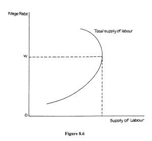
Figure 8.6

• Like any other economic good, the supply of labour is influenced by price – the wage rate. Clearly this has a major impact on the supply of labour to particular occupations and industries.  Other things being equal (which they rarely are) people generally prefer to work in the more highly-paid sectors of employment.  However, the impact of the general wage rate on the total supply of labour is less certain.  People work to obtain income.  They also need free time, given the general term “leisure”, in order to enjoy that income.  Consequently, there is always something of a conflict between the need to work to gain income and the desire for leisure.  High income and little leisure can be as unsatisfactory as a great deal of leisure and little income.  The widely accepted view among economists is that people can be expected to wish to work more as wage rates rise from low levels, but that there comes a point when the desire for leisure becomes more powerful than the desire for more income and the response to any further rise in the wage rate is to work less.  There is much evidence to suggest that people have a target level of income according to their view of what constitutes a satisfactory living standard, and once that target is reached, they prefer to have increased time of their own.  The target can, of course, change as the purchasing power of money and people’s expectations and ambitions change.  However, the implication of this view of people’s attitudes to work, income and leisure is that the supply of labour curve is likely to slope backwards at the higher wage levels, as illustrated in Figure 8.6.  When the wage rate reaches Ow, the preference for leisure becomes more powerful than the desire for additional income, so the total supply of labour starts to fall when wages rise above this level.
• There is also firm evidence that this shaped supply of labour curve appears to apply to men more than to women. It seems that, at current wage levels, the supply of female labour continues to rise with the level of wages. A number of explanations have been offered for this difference between the attitudes of men and women.  These include:
  • Where families cannot help, many women incur expense in securing child care and house cleaning services when they decide to remain in or return to the workforce. Only those women whose incomes from working exceed the cost of working can afford to work.  As wage rates rise, more women fall into this group.
  • Household income often depends on the combined incomes of a man and woman in the household. At low wage levels, reliance is chiefly on the man’s income, but as wage rates rise, the man may decide to take more “leisure” in order to help with the family and home so that the woman can return to work.
  • The general desire of women to work has been so strong during the past two or three decades for a mixture of financial and non-financial reasons, that it has resulted in a continued increase in female employment during the time that wage levels have been rising. Statistically it is difficult to separate the wage from the non-wage influences when there is this strong trend in one direction.  The supply-side pressures have been matched by the employers’ demand for part-time female workers as one way to bring greater flexibility into the workforce in a period when socially and politically inspired employment protection legislation has been making it more rigid in spite of increased competition and insecurity in product markets.

Factors Influencing Labour Supply

• Society, Laws and Customs
• Labour Immobility. (i.e. restrictions on labour movement)
  • between regions and countries (= geographic immobility)
  • between jobs (i.e. occupational immobility) caused by – union barriers, professional barriers, lack of information on job opportunities, housing shortages (expense, non-monetary considerations (friends, social life), ability, linguistic and cultural differences.)
• Barriers of entry to certain professions/trades (e.g. professional qualifications, long apprenticeship)
• Lack of freely-available information about jobs and wages. (e) Trade Union influence on labour supply and wages.

Trade unions can have a significant influence on wage levels.

The Bargaining Theory of Wages: is that wage levels are set by negotiation between unions and management by a process of Collective Bargaining.

The role of unions is to raise the real wage of the work force by:

• Erect and maintain barriers to entry into jobs so as to ensure high earnings for existing members.
• Monopolise the supply of labour in the industry.

However, unions cannot go on raising the real wages of the work force unless labour increases its productivity (output per worker) so as to offset the increase in its costs.

Methods Used By Trade Unions

• Negotiations with employers (generally annual).
• Official Strikes.
• Picketing
• Work to Rule or Go-Slow or overtime ban.
• Selective Strike Action.
• Unofficial Strikes.
• National Wage Agreements –e. wage agreements negotiated at a national level between trade union and employers’ federations. This sets a minimum or “normal” wage level or wage rise firms can then negotiate around that “norm” with their own employees.
• Minimum Wages – minimum legal wage that all workers must receive. It is used to protect the incomes of the lower paid and thus is used as a means of relieving poverty. There are arguments made for and against minimum wage legislation. The main argument against it is that it reduces employment as some firms cannot afford to pay the higher wage. Another is that it does little to reduce poverty among those who do not work as it only benefits those in employment.

Sources of Unions Depends on:

• The union’s size, financial resources and negotiating skills.
• The sensitivity of its workers’ occupations (e.g. electricity worker’s strike can have a huge impact).
• A union’s ability to control the supply of labour (closed-shop helps).
• Economic viability of the industry.
• General Economic Conditions.
• A union’s relationship with the government. (vii) Technological progress (ix) Restrictive wage legislation.
• Market Conditions.
• Labour Productivity Improvements. Wage Differentials

These are differences in the rate of pay between one type of job and another.

Wage Differentials depend on:

• Restrictions on supply of certain types of labour (e.g. because of professional `      qualifications, rare abilities, danger).
• Higher demand for certain types of labour.
• Higher revenue for certain occupations.
• Union Strength in different occupations.

Skilled workers tend to be paid more than unskilled because:

• They are more productive (i.e. have a higher Product of Labour).
• They are scarcer (i.e. demand is less relative to supply, so their supply curve is further to the left).
• Supply of skilled workers is relatively INELASTIC because of barriers to entry (professional qualifications) and because availability of people with suitable talent is restricted.

Wages differentials could be eroded by (a) Strike action.

• Minimum wage legislation.
• Income controls
• Increased productivity by unskilled workers.
• Training incentives.

Functions of Factor Markets

The factor market performs two functions, as follows:

• Rationing: the supply of factors is rationed between the users so that the greatest supply is given to those best able to use the factor efficiently, as shown by their ability to pay the highest price for the factor.
• Distribution: factors are directed to those areas of production where they are most valuable.  These will be areas which are best able to pay high rewards.  This ability to pay will result from the fact that these are areas where demand for consumer products is highest.  Thus, the distribution of factors is determined by the demand for consumer and investment goods and services.

In the modern mixed economy, however, markets are seldom perfect, and we have to recognise that non-economic motives are sometimes important.  We also have to recognise the importance of government influence.  We shall see that some types of labour and land are largely outside the price system, although they are rarely altogether unaffected by it.

Business Demand for Factors

The demand for production factors is what is often called a “derived demand”.  This is because the firm will employ factors only as long as they contribute to the profits of the organisation.  A factor is wanted because it is necessary for the production of the firm’s product, and the firm’s profit comes from selling its product.

In general, therefore, the higher the demand for the firm’s product, the greater will be its ability to make profits, and the more factors it will want to employ.

However, the demand for factors may not rise in direct proportion to any rise in the demand for the product, because the firm will try to make more efficient use of the factors it already has, before it employs more.  Thus, a 10% rise in the demand for the product is likely to lead to a less than 10% increase in factor demand.  In a period of very rapid technological advance there might have to be a very great increase in product demand indeed to produce any really significant increase in total factor demand.  In particular, developments in electronics and what may be termed “micro-technology” mean that the demand for space or land is not likely to increase in anything like the same proportion as production increases.  Many machines have become smaller, as well as more efficient.  Micro-computers take up much less space than mainframe computers.

The main interest of economists, however, tends to be concentrated on the relative demand for capital and labour – machines and people – because these are to a very large extent substitutes for each other and, of course, the employment or unemployment of people has very important social implications.  The firm’s desire to employ machines or people, and the proportions in which they are employed, depends on the extent to which they can contribute to production.  If, for example, a machine can produce twice as much as a man, for the same yearly cost, then the employer will prefer to employ the machine, other things being equal.  If we recognise this simple fact, then we can see that the demand for labour in relation to the demand for capital (machinery) will depend on:

• The productivity of both labour and capital – i.e. the amount that each can add to total production per unit; and
• the unit price of both labour and capital.

If the firm is seeking to maximise profits, then it will try to aim at the condition where the additional product contributed by the last RWF spent on labour will be exactly equal to the additional product contributed by the last RWF spent on capital (equipment/machines, etc.).

If this is not the position, then the firm can increase its efficiency and profitability by switching from labour to capital, or vice versa, according to which offers the greater increase in production for each RWF of additional expenditure.  If the extra production per RWF of labour is two units and the extra achieved by spending another RWF on capital is four units, then clearly the firm will gain by spending fewer RWFs on labour, and more RWFs on capital.

We can express precisely this idea more formally in the equation.

 

^MPPL ₌^MPPK                where     MPP_L    = the marginal physical product of labour

P_L                 PK

MPP_K    = the marginal physical product of capital

 

P_L           = the unit price of labour P_K           = the unit price of capital

The marginal physical product of a factor is the addition to the total product achieved by employing one more unit of the factor – in the reduction in total product suffered by employing one less unit of the factor.

Factor markets are not perfect, and a firm’s ability to achieve this condition is likely to be constrained by a number of influences, including labour law, trade union power, and the fact that there are what are called indivisibilities in the employment of factors.  For example, if one worker is needed to look after three machines, the firm cannot employ 1 workers if it wishes to use five machines.  It is likely to need two workers but will then have excess labour capacity, and will have a strong incentive to increase its product sales in order to justify acquiring the sixth machine which will add nothing to labour costs.

However, even if the firm is unlikely to be able to achieve the profit-maximising ideal employment of factors, this analysis shows us which employment trends are likely to follow certain relative changes in productivity and prices of labour and capital.

If technological advances produce more productive and cheaper machines, and trade unions achieve higher real wages and “improved working conditions” – which often means reduced labour productivity – then we cannot be surprised if, after a time, business demand for capital rises while demand for labour falls, and there is a rise in worker unemployment.

 ECONOMIC RENT

Meaning of Economic Rent

It is a feature of all markets, but especially true of factor markets, that the market price is determined briefly by conditions at the margin.  In the absence of price discrimination, all buyers pay the price which reflects the utility of the marginal or last buyer.  Similarly, all workers in a firm are usually paid the same wage as that paid to the last one employed in that category.  If the last worker to be employed was paid more than the others, then all the others could leave and seek re-employment at that marginal rate.  The same principle applies to other factors of production.  If we accept this, then we can see that, at any given time, most factors will be employed at a rate that is above the lowest rate which would bring them into the market.  If, for example, worker A joins a firm at a wage of RWF100 per week and if, in the course of time, the firm expands and takes on more workers and, to attract more workers it has to raise the wage to, say, RWF120, then the worker who joined the firm for RWF100 is getting RWF20 more than the amount at which he would still be prepared to be employed in that work.  (Inflation is, of course, ignored here, and we assume that money values are constant over time.)  The extra RWF20 is the result of the operation of the market and of the interplay of the economic forces of supply and demand.  As such, it is termed economic rent.

The term may seem confusing as applied to workers, but the concept was originally worked out in respect of land – hence “rent”.  At the time, people were blaming the rising prices of food on greedy landlords who were demanding increased rents for their land.  Some economists of the day pointed out that it was the rising demand for food from a growing and increasingly urban population that was pushing up food prices and bringing into production more land at increased rents.  Because the poorer marginal land was able to command higher rents, the rents of other productive land also rose, even though their use did not change.  The owners of the land which had always been in use gained an economic rent over and above the rent at which they would still have farmed their land.

Economic Rent in the Market

The idea of economic rent applies to all factors in the market as a whole, and is only zero for the marginal factor just attracted into the market at the current rate.  The diagram in Figure 8.7 is often used to illustrate this.  From it we see that the market equilibrium wage is Ow, and this is the wage paid to all workers in that market.  Notice that the supply of labour curve reflects the probability that there is a minimum wage below which no one is prepared to work in that market.  Ow is the wage needed to attract into the market the marginal worker at OL.  All other workers would be prepared to enter the market at a lower wage – this being illustrated by the existence of a supply-of-labour curve.  The amount at which each worker is prepared to enter or remain in the market is likely to be determined by the next-best wage he could obtain elsewhere, and is thus known as the “transfer earnings” (earnings received on transfer to the next-best market).

 

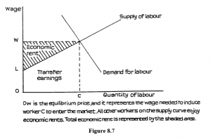
Figure 8.7

Thus, all workers in the market and receiving wage Ow, other than the marginal worker, are receiving part transfer earnings and part economic rent.  The total amount of economic rent in the market is represented by the shaded area.  The area below the supply curve up to quantity OL is total transfer earnings.

Economic Rent and the Individual

The position of the individual worker (or other factor) in the market is illustrated in Figure 8.8.  Here again, the market equilibrium wage resulting from the interaction of demand and supply is Ow.  Worker “a” receives the market wage Ow but his position on the supply curve indicates that he would enter or remain in the market at the lower wage of OWa.

Thus, the amount W-Wa represents the proportion of his total wage that is economic rent.  His next-best earnings are Ow.

The concept is important in the analysis of wages, because it suggests that workers whose wage contains a high element of economic rent are very vulnerable to changes in market conditions that would reduce the equilibrium wage.  That money wages have not fallen in the industrial nations for most of the past half century does not mean that they cannot fall – or, indeed, should not fall, under certain conditions.

What has happened in recent years is that demand has fallen in many labour markets, and this has affected real wages, i.e. money wages adjusted to take account of changes in the purchasing power of money.  This readjustment has not only reduced the amount of economic rent in those markets, but has also forced those workers who have had to leave the market to discover that their transfer earnings were much lower than their previous wage.  Those workers who have sought to obtain work at a level close to their old wage, instead of accepting it at their transfer earnings rate, have usually remained unemployed.

 

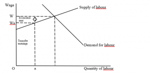
Figure 8.8

The implication for the individual worker is very clear.  The greater the element of economic rent in the current wage, the greater the degree of vulnerability to any change in market conditions.  The worker least likely to suffer is the one with the least economic rent and the highest level of transfer earnings.  Thus, workers with several marketable skills, those able to retrain to meet demand in new markets, are the ones with the lowest economic rent, and they have the least to fear from economic change.

Quasi-Rent

The term quasi-rent is sometimes used to describe a form of economic rent for a factor the supply of which is temporarily highly inelastic or completely fixed.  The use of “quasi” indicates that, in the long run, supply is not fixed.

Take the case of a sport which becomes popular very quickly.  The few people who are star performers at the time of the popularity surge, suddenly become well known and in great demand for competitions and “appearances”.  Their earnings rise very quickly but contain a high rent element.  These high earnings attract to the sport talented people who had not previously considered a serious career in it.  The standard of performances increases, as does the number of star performers.  Only those with most exceptional talent are now able to earn very high incomes.  Others, who would have been stars by the standards of a few years earlier, can earn little more than an average income.

The situation is illustrated in Figure 8.9.  As people respond to the increased earnings possibilities, the supply curve swings to the right at this higher earnings level, and the extent of economic rent is reduced, as shown in the model.

 

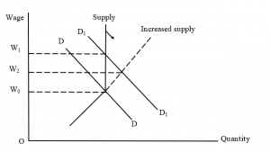
Figure 8.9

Supply totally inelastic in the short term and, following a rise in demand DD to D₁D₁, the wage rises from Ow_o to Ow₁.  There is economic rent of W₁-W_o.  In time, and in response to the increased rewards, supply rises and the economic rent element falls bringing down the wage to Ow₂.