FINANCIAL STATEMENT ANALYSIS – MASOMO MSINGI PUBLISHERS

INTRODUCTION

The management, creditors, investors and others use the information contained in the statements of changes in financial position (funds and cash flow statements) to form judgment about the operating performance and financial position of the firm. Users of financial statements can get further insight about financial strengths and weaknesses of the firm if they properly analyse information reported in these statements. Management should be particularly interested in knowing financial strengths of the firm to make their best use and to be able to spot out financial weaknesses of the firm to take suitable corrective actions. The future plans of the firm should be laid down in view of the firm’s financial strengths and weaknesses. Thus, financial analysis is the starting point for making plans, before using any sophisticated forecasting and planning procedures.

Understanding the past is a prerequisite for anticipating the future.

USERS OF FINANCIAL ANALYSIS

Financial analysis is the process of identifying the financial strengths and weaknesses of the firm by properly establishing relationships between the items of the balance sheet and the profit and loss account. Financial analysis can be undertaken by the management of the firm, or by parties outside the firm, viz., owners, creditors, investors and others.¹ The nature of analysis will differ depending on the purpose of the analyst.

Trade creditors are interested in a firm’s ability to meet their claims over a very short period of time. Their analysis will, therefore, confine to the evaluation of the firm’s liquidity position.
Suppliers of long-term debt, on the other hand, are concerned with the firm’s longterm solvency and survival. They analyze the firm’s profitability over time, its ability to generate cash to be able to pay interest and repay principal, and the relationship between various sources of funds (capital structure relationships). Long-term creditors do analyze the historical financial statements, but they place more emphasis on the firm’s projected, or pro forma, financial statements to make analysis about its future solvency and profitability.
Investors, who have invested their money in the firm’s shares, are most concerned about the firm’s earnings. They restore more confidence in those firms that show steady growth in earnings. As such, they concentrate on the analysis of the firm’s present and future profitability. They are also interested in the firm’s financial structure to the extent it influences the firm’s earnings ability and risk.
Management of the firm would be interested in every aspect of the financial analysis. It is their overall responsibility to see that the resources of the firm are used most effectively and efficiently, and that the firm’s financial condition is sound.

Check Your Concepts

1. What is meant by financial analysis?

2. Who uses financial analysis and for what?

NATURE OF RATIO ANALYSIS

Ratio analysis is a powerful tool of financial analysis. A ratio is defined as “the indicated quotient of two mathematical expressions” and as “the relationship between two or more things.”² In financial analysis, a ratio is used as a benchmark for evaluating the financial position and performance of a firm. The absolute accounting figures reported in the financial statements do not provide a meaningful understanding of the performance and financial position of a firm. An accounting figure conveys meaning when it is related to some other relevant information. For example, a `5 crore net profit may look impressive, but the firm’s performance can be said to be good or bad only when the net profit figure is related to the firm’s investment. The relationship between two accounting figures, expressed mathematically, is known as a financial ratio (or simply as a ratio). Ratios help to summarize large quantities of financial data and to make qualitative judgment about the firm’s financial performance. For example, consider current ratio (discussed in detail later on). It is calculated by dividing current assets by current liabilities; the ratio indicates a relationship—a quantified relationship between current assets and current liabilities. This relationship is an index or yardstick, which permits a qualitative judgment to be formed about the firm’s ability to meet its current obligations. It measures the firm’s liquidity. The greater the ratio, the greater is the firm’s liquidity and vice versa. The point to note is that a ratio reflecting a quantitative relationship helps to form a qualitative judgment. Such is the nature of all financial ratios.

Standards of Comparison

The ratio analysis involves comparison for a useful interpretation of the financial statements. A single ratio in itself does not indicate favourable or unfavourable condition. It should be compared with some standard. Standards of comparison may consist of:³

past ratios, i.e., ratios calculated from the past financial statements of the same firm;
competitors’ ratios, i.e., ratios of some selected firms, especially the most progressive and successful competitor, at the same point in time;
industry ratios, i.e., ratios of the industry to which the firm belongs; and
projected ratios, i.e., ratios developed using the projected, or pro forma, financial statements of the same firm.

Time series analysis The easiest way to evaluate the performance of a firm is to compare its present ratios with the past ratios. When financial ratios over a period of time are compared, it is known as the time series analysis. It gives an indication of the direction of change and reflects whether the firm’s financial performance has improved, deteriorated or remained constant over time. The analyst should not simply determine the change, but, more importantly, he/she should understand why ratios have changed. The change, for example, may be affected by changes in the accounting policies without a material change in the firm’s performance.

Cross-sectional analysis Another way of comparison is to compare ratios of one firm with some selected firms in the same industry at the same point in time. This kind of comparison is known as the cross-sectional analysis or inter-firm analysis. In most cases, it is more useful to compare the firm’s ratios with ratios of a few carefully selected competitors, who have similar operations. This kind of a comparison indicates the relative financial position and performance of the firm. A firm can easily resort to such a comparison, as it is not difficult to get the published financial statements of the similar firms.

Industry analysis To determine the financial condition and performance of a firm, its ratios may be compared with average ratios of the industry of which the firm is a member. This sort of analysis, known as the industry analysis, helps to ascertain the financial standing and capability of the firm vis-à-vis other firms in the industry. Industry ratios are important standards in view of the fact that each industry has its characteristics, which influence the operating relationships. But there are certain practical difficulties in using the industry ratios. First, it is difficult to get average ratios for the industry. Second, even if industry ratios are available, they are averages—averages of the ratios of strong and weak firms. Sometimes differences may be so wide that the average may be of little utility. Third, averages will be meaningless and the comparison futile if firms within the same industry widely differ in their accounting policies and practices. If it is possible to standardize the accounting data for companies in the industry and eliminate extremely strong and extremely weak firms, the industry ratios will prove to be very useful in evaluating the relative financial condition and performance of a firm.

Pro forma analysis Sometimes future ratios are used as the standard of comparison. Future ratios can be developed from the projected, or pro forma financial statements. The comparison of current or past ratios with future ratios shows the firm’s relative strengths and weaknesses in the past and the future. If the future ratios indicate weak financial position, corrective actions should be initiated.

Types of Ratios

Several ratios, calculated from the accounting data, can be grouped into various classes according to the financial activity or function to be evaluated. As stated earlier, the parties interested in financial analysis are short- and long-term creditors, owners and management. Short-term creditors’ main interest is in the liquidity position or the short-term solvency of the firm. Long-term creditors, on the other hand, are more interested in the long-term solvency and profitability of the firm. Similarly, owners concentrate on the firm’s profitability and financial condition. Management is interested in evaluating every aspect of the firm’s performance. They have to protect the interests of all parties and see that the firm grows profitably. In view of the requirements of the various users of ratios, we may classify them into the following four important categories:⁴

Liquidity ratios
Leverage ratios
Activity ratios
Profitability ratios

Liquidity ratios measure the firm’s ability to meet current obligations, leverage ratios show the proportions of debt and equity in financing the firm’s assets, activity ratios reflect the firm’s efficiency in utilizing its assets and profitability ratios measure overall performance and effectiveness of the firm. Each of these ratios is discussed below. The accounting data are taken from the financial statements for the Hindustan Manufacturing Company (the real name of the company has been disguised) to illustrate calculation and use of ratios.

Check Your Concepts

1. What is meant by financial ratio?

2. What are the types of ratios most commonly used in financial analysis? What does each type of theratios measure?

3. With reference to ratio analysis, explain the following: (a) time series analysis, (b) cross-section analysis, (c) industry analysis, (d) pro forma analysis.

ILLUSTRATION 20.1: Assessing Financial Health of a Firm with Ratio Analysis

The Hindustan Manufacturing Company is a leading producer and exporter of engineering items such as steel pipes, ingots, billets, etc. It has also recently added a chemical plant and a paper plant as part of its diversification strategy. The company started with a share capital of `25 lakh in the early sixties, which has now increased to `225 lakh. The number of shares outstanding is 22.50 lakh. The average market price (AMP) of the company’s share during 20X1–20X3 has been: `26.38 in 20X1, `34.50 in 20X2 and `29.25 in 20X3. The financial data for the company are given in Tables 20.1 to 20.3. For illustrative purpose, calculations of ratios have been shown only for the year 20X3. However, tables indicating trend in ratios during 20X1–20X3 are also given.

Table 20.1: Hindustan Manufacturing Company

Profit and Loss Account

for the year ending on 31 March (` lakh)

		20X1	20X2	20X3
A.	Net sales*	2,338.90	2,825.69	3,717.23
B.	Cost of goods sold**	1,929.04	2,322.80	3,053.66
C.	Gross profit (A – B)	409.86	502.89	663.57
D.	Less: Selling and adm. expenses	239.72	262.10	357.87
E.	Operating income (C – D)	170.14	240.79	305.70
F.	Add: Other income	15.24	25.38	36.91
G.	Earning before int. and tax (EBIT) (E + F)	185.38	266.17	342.61
H.	Less: Interest	59.84	124.98	143.46
I.	Profit before tax (PBT) (G – H)	125.54	141.19	199.15
J.	Provision for tax	41.79	30.00	64.29
K.	Profit after tax (PAT) (I – J)	83.75	111.19	134.86
L.	Effective tax rate***	33%	21%	32%
M.	Dividend distributed	33.75	39.38	45.00
N.	Retained earnings	50.00	71.81	89.86

* Net of excise duty.

** Depreciation included.

*** Provision for tax divided by profit before tax.

Table 20.2: Hindustan Manufacturing Company Statement of Cost of Goods Sold

for the year ending on March 31 (` lakh)

	20X1 20X2 20X3
Raw material	1,587.34 2,019.54 2,751.52
Direct labour	138.13 170.86 228.94
Depreciation	23.07 38.64 41.59
Other mfg. expenses	205.34 255.72 329.44 1,953.88 2,484.76 3,351.49
Add: Opening stock in process	57.09 85.74 150.55 2,010.97 2,570.50 3,502.04
Less: Closing stock in process	85.74 150.55 230.83
Cost of Production	1,925.23 2,419.95 3,271.21
Add: Opening finished stock	150.93 147.12 244.26 2,076.16 2,567.07 3,515.47
Less: Closing finished stock	147.12 244.26 461.81
Cost of Goods Sold	1,929.04 2,322.81 3,053.66

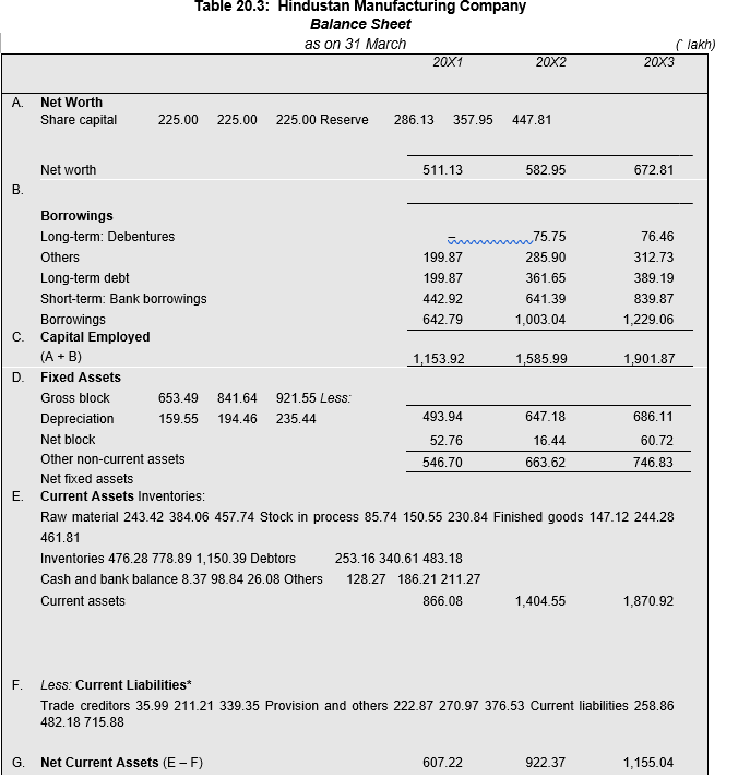
H.	Net Assets (D + G) 1,153.92 1,585.99 1,901.87

* If bank borrowings are considered, then the current liabilities for 20X1 through 20X3 will be: `701.78 lakh; `1123.57 lakh, and `1555.75 lakh.

LIQUIDITY RATIOS

It is extremely essential for a firm to be able to meet its obligations as they become due. Liquidity ratios measure the ability of the firm to meet its current obligations (liabilities). In fact, analysis of liquidity needs the preparation of cash budgets and cash and fund flow statements; but liquidity ratios, by establishing a relationship between cash and other current assets to current obligations, provide a quick measure of liquidity. A firm should ensure that it does not suffer from lack of liquidity, and also that it does not have excess liquidity. The failure of a company to meet its obligations due to lack of sufficient liquidity will result in a poor credit worthiness, loss of creditors’ confidence or even in legal tangles resulting in the closure of the company. A very high degree of liquidity is also bad; idle assets earn nothing. The firm’s funds will be unnecessarily tied up in current assets. Therefore, it is necessary to strike a proper balance between high liquidity and lack of liquidity.

The most common ratios, which indicate the extent of liquidity or lack of it, are: (i) current ratio and (ii) quick ratio. Other ratios include cash ratio, interval measure and networking capital ratio.

Current Ratio

Current ratio is calculated by dividing current assets by current liabilities:

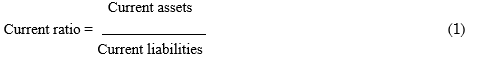
Current assets include cash and those assets that can be converted into cash within a year, such as marketable securities, debtors and inventories. Prepaid expenses are also included in current assets as they represent the payments that will not be made by the firm in the future. All obligations maturing within a year are included in current liabilities. Current liabilities include creditors, bills payable, accrued expenses, short-term bank loan, income-tax liability and longterm debt maturing in the current year.

The current ratio is a measure of the firm’s short-term solvency. It indicates the availability of current assets in rupees for every one rupee of current liability. A ratio of greater than one means that the firm has more current assets than current claims against them.

For HMC, the current ratio is:

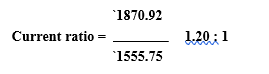
How to interpret current ratio? As a conventional rule, a current ratio of 2 to 1 or more is considered satisfactory. The Hindustan Manufacturing Co. has a current ratio of 1.20:1; therefore, it may be interpreted to be insufficiently liquid. This rule is based on the logic that in a worse situation, even if the value of current assets becomes half, the firm will be able to meet its obligation. The current ratio represents a margin of safety for creditors. The higher the current ratio, the greater the margin of safety; the larger the amount of current assets in relation to current liabilities, the more the firm’s ability to meet its current obligations. However, an arbitrary standard of 2 to 1 should not be blindly followed. Firms with less than 2 to 1 current ratio may be doing well, while firms with 2 to 1 or even higher current ratios may be struggling to meet their obligations. This is so because the current ratio is a test of quantity, not quality. The current ratio measures only total rupees’ worth of current assets and total rupees’ worth of current liabilities. It does not measure the quality of assets. Liabilities are not subject to any fall in value; they have to be paid. But current assets can decline in value. If the firm’s current assets consist of doubtful and slow-paying debtors or slow-moving and obsolete stock of goods, then the firm’s ability to pay bills is impaired; its short-term solvency is threatened. Thus, too much reliance should not be placed on the current ratio; a further investigation about the quality of the items of current assets is necessary. However, the current ratio is a crude-and-quick measure of the firm’s liquidity.

Quick Ratio

Quick ratio, also called acid-test ratio, establishes a relationship between quick, or liquid, assets and current liabilities. An asset is liquid if it can be converted into cash immediately or reasonably soon without a loss of value. Cash is the most liquid asset. Other assets that are considered to be relatively liquid and included in quick assets are debtors and bills receivable, and marketable securities (temporary quoted investments). Inventories are considered to be less liquid.

Inventories normally require some time for realizing into cash; their value also has a tendency to fluctuate. The quick ratio is found out by dividing quick assets by current liabilities.

Thus, if the HMC’s inventories do not sell, and it has to pay all its current liabilities, it may find it difficult to meet its obligations because its quick assets are 0.46 times of current liabilities.

Is quick ratio a better measure of liquidity? Generally, a quick ratio of 1 to 1 is considered to represent a satisfactory current financial condition. Although quick ratio is a more penetrating test of liquidity than the current ratio, yet it should be used cautiously. A quick ratio of 1 to 1 or more does not necessarily imply sound liquidity position. It should be remembered that all debtors may not be liquid, and cash may be immediately needed to pay operating expenses. It should also be noted that inventories are not absolutely non-liquid. To a measurable extent, inventories are available to meet current obligations. Thus, a company with a high value of quick ratio can suffer from a shortage of funds if it has slow paying, doubtful and long-duration outstanding debtors. On the other hand, a company with a low value of quick ratio may really be prospering and paying its current obligation in time if it has been turning over its inventories efficiently. Nevertheless, the quick ratio remains an important index of the firm’s liquidity.

Cash Ratio

Since cash is the most liquid asset, a financial analyst may examine cash ratio and its equivalent to current liabilities. Trade investment or marketable securities are equivalent of cash; therefore, they may be included in the computation of cash ratio:

The company in our example carries a small amount of cash. There is nothing to be worried about the lack of cash if the company has reserve borrowing power. In India, firms have credit limits sanctioned from banks, and can easily draw cash.

Interval Measure

Yet another ratio, which assesses a firm’s ability to meet its regular cash expenses, is the interval measure. Interval measure relates liquid assets to average daily operating cash outflows. The daily operating expenses will be equal to the cost of goods sold plus selling, administrative and general expenses less depreciation (and other non-cash expenditures) divided by number of days in the year (normally 360).

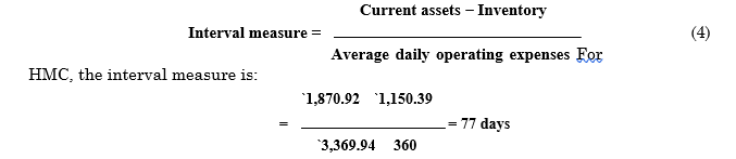
For HMC, interval measure indicates that it has sufficient liquid assets to finance its operations for 77 days, even if it does not receive any cash.

Interval measure may be refined further. Instead of calculating only the daily operating expenditures, one may also include expenditures required for paying interest, acquiring assets and repaying debt.

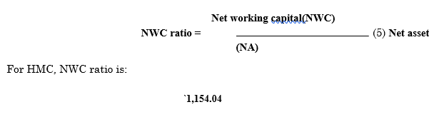
Net Working Capital Ratio

The difference between current assets and current liabilities excluding short-term bank borrowing is called net working capital (NWC) or net current assets (NCA). NWC is sometimes used as a measure of a firm’s liquidity. It is considered that, between two firms, the one having the larger NWC has the greater ability to meet its current obligations. This is not necessarily so; the measure of liquidity is a relationship, rather than the difference between current assets and current liabilities. NWC, however, measures the firm’s potential reservoir of funds. It can be related to net assets (or capital employed):

Table 20.4 presents the three-year trend of HMC’s liquidity ratios.

Table 20.4: Hindustan Manufacturing Company

Liquidity Ratios

	20X1	20X2	20X3
Current ratio	1.24	1.25	1.20
Quick ratio	0.56	0.56	0.46
Cash ratio	0.01	0.09	0.02
Interval measure (days)	65.00	87.00	77.00
Net working capital ratio	0.53	0.58	0.61

Ratios in Table 20.4 indicate that HMC’s liquidity is deteriorating. A note of caution may be sounded: liquidity ratio can mislead since current assets and current liabilities can change quickly. Their utility becomes more doubtful for firms with seasonal business. In the case of seasonal businesses, liquidity ratios from quarterly or monthly financial data would be more appropriate.

Check Your Concepts

1. What is meant by liquidity ratio? What are the types of liquidity ratios?

2. How are the following ratios calculated: (a) current ratio; (b) quick ratio; (c) cash ratio; (d) net working capital ratio; (e) interval measure?

3. What is the utility of liquidity ratios?

LEVERAGE RATIOS

The short-term creditors, like bankers and suppliers of raw material, are more concerned with the firm’s current debt-paying ability. On the other hand, long-term creditors, like debenture holders, financial institutions, etc., are more concerned with the firm’s long-term financial strength. In fact, a firm should have a strong short-as well as long-term financial position. To judge the long-term financial position of the firm, financial leverage, or capital structure ratios are calculated. These ratios indicate mix of funds provided by owners and lenders. As a general rule, there should be an appropriate mix of debt and owners’ equity in financing the firm’s assets.

The manner in which assets are financed has a number of implications. First, between debt and equity, debt is more risky from the firm’s point of view. The firm has a legal obligation to pay interest to debt holders, irrespective of the profits made or losses incurred by the firm. If the firm fails to pay to debt holders in time, they can take legal action against it to get payments and in extreme cases, can force the firm into liquidation. Second, use of debt is advantageous for shareholders in two ways: (a) they can retain control of the firm with a limited stake and (b) their earning will be magnified when the firm earns a rate of return on the total capital employed higher than the interest rate on the borrowed funds. The process of magnifying the shareholders’ return through the use of debt is called ‘financial leverage’ or ‘financial gearing’ or ‘trading on equity.’ However, leverage can work in opposite direction as well. If the cost of debt is higher than the firm’s overall rate of return, the earnings of shareholders will be reduced. In addition, there is threat of insolvency. If the firm is actually liquidated for non-payment of debt-holders’ dues, the worst sufferers will be shareholders—the residual owners. Thus, use of debt magnifies the shareholders’ earnings as well as increases their risk. Third, a highly debt-burdened firm will find difficulty in raising funds from creditors and owners in future. Creditors treat the owners’ equity as a margin of safety; if the equity base is thin, the creditors risk will be high. Thus, leverage ratios are calculated to measure the financial risk and the firm’s ability of using debt to shareholders’ advantage.

Leverage ratios may be calculated from the balance sheet items to determine the proportion of debt in total financing. Many variations of these ratios exist; but all these ratios indicate the same thing—the extent to which the firm has relied on debt in financing assets. Leverage ratios are also computed from the profit and loss items by determining the extent to which operating profits are sufficient to cover the fixed charges.

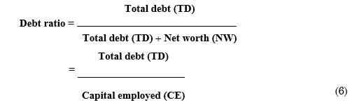
Debt Ratio

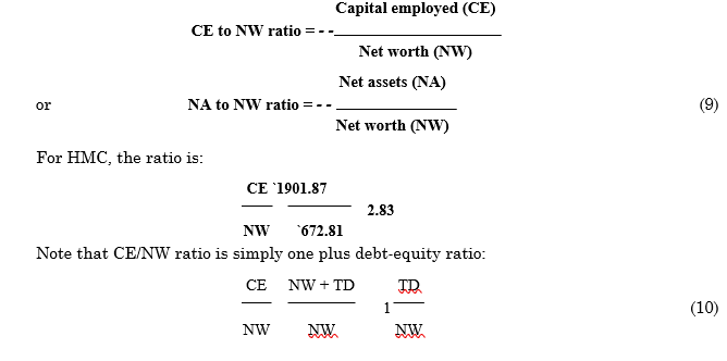
Several debt ratios may be used to analyze the long-term solvency of a firm. The firm may be interested in knowing the proportion of the interest-bearing debt (also called funded debt) in the capital structure. It may, therefore, compute debt ratio by dividing total debt (TD) by capital employed (CE) or net assets (NA). Total debt will include short and long-term borrowings from financial institutions, debentures/bonds, deferred payment arrangements for buying capital equipments, bank borrowings, public deposits and any other interest-bearing loan. Capital employed will include total debt and net worth (NW).

Note that capital employed (CE) equals net assets (NA) that consist of net fixed assets (NFA) and net current assets (NCA). Net current assets are current assets (CA) minus current liabilities (CL) excluding interest-bearing short-term debt for working capital. These relationships are:

NFA  CA  NW  TD  CL

NFA  CA  CL  NW  TD

NFA  NCA NW  TD

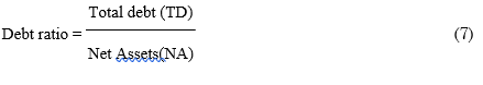
NA  CE

Because of the equality of capital employed and net assets, debt ratio can also be defined as total debt divided by net assets:

For HMC, the ratio is:

`389.19 + `839.87

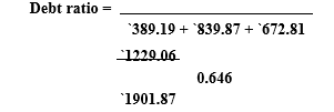
The debt ratio of 0.646 means that lenders have financed 64.6 per cent or about two-thirds of HMC’s net assets (capital employed). It obviously implies that owners have provided the remaining finances. They have financed: 1 – 0.646 = 0.354 = 35.4 per cent or about one-third of net assets.

Debt-Equity Ratio

It is clear that from the total debt ratio that HMC’s lenders have contributed more funds than owners; lenders’ contribution is 1.83 times of owners’ contribution, viz., 0.646/0.354 = 1.83. This relationship describing the lenders’ contribution for each rupee of the owners’ contribution is called debt-equity ratio. Debt-equity (DE) ratio is directly computed by dividing total debt by net worth:

Capital employed to net worth ratio There is yet another alternative way of expressing the basic relationship between debt and equity. One may want to know: How much funds are being contributed together by lenders and owners for each rupee of the owners’ contribution? Calculating the ratio of capital employed or net assets to net worth can find this out:

Other Debt Ratios

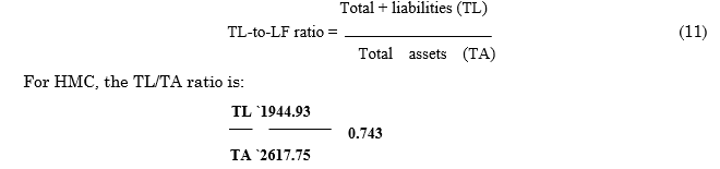
Current liabilities (non-interest bearing current obligations) are generally excluded from the computation of leverage ratios. One may like to include them on the ground that they are important determinants of the firm’s financial risk since they represent obligations and exert pressure on the firm and restrict its activities. Thus, to assess the proportion of total funds—short and long term— provided by outsiders to finance total assets, the following ratio may be calculated:

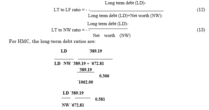
In addition to debt ratios explained so far, a firm may wish to calculate leverage ratios in terms of the long-term capitalization or funds (LTF) alone. Long-term funds or capitalization will include long-term debt and net worth. Thus, the firm may calculate the following long-term debt ratios

How to treat preference capital? Some firms have preference share capital in their capital structure. How should it be treated in computing leverage ratios? Whether the preference capital will be included in debt or net worth will depend on the purpose for which the leverage ratio is being calculated. If it is calculated to show the effect of leverage on the ordinary (or common) shareholders’ earnings, the preference capital should be included in debt. The preference dividend is fixed like the interest cost and the ordinary shareholders’ earnings will be magnified if the rate of preference dividend is less than the firm’s overall rate of return. But if the leverage ratio is calculated to reflect the financial risk, the preference capital should be included in net worth. ‘The treatment of preference share capital as debt ignores the fact that debt and preference share capital present different risk to shareholders. In one case failure to meet payments means bankruptcy and possible elimination of the common shareholders, while in the other case failure to meet payments presents no such risk.’⁵In the financial analysis, leverage is seen to reflect the financial risk; therefore, preference capital should be included in net worth.

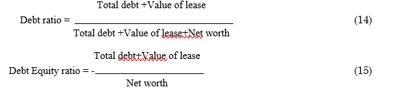
How to treat lease payments? When a company obtains the use of fixed assets under long-term lease agreements, it commits itself to a series of fixed payments (viz., lease rentals). The value of lease obligations is thus equivalent to debt. It is, therefore, natural to include the capitalized value of lease obligation in debt while measuring the firm’s financial leverage:

What do debt ratios imply? Whatever way the debt ratio is calculated, it shows the extent to which debt financing has been used in the business. A high ratio means that claims of creditors are greater than those of owners. A high level of debt introduces inflexibility in the firm’s operations due to the increasing interference and pressures from creditors. A high-debt company is able to borrow funds on very restrictive terms and conditions. The loan agreements may require a firm to maintain a certain level of working capital, or a minimum current ratio, or restrict the payment of dividends, or fix limits to the officers’ and employees’ salaries and so on. Heavy indebtedness leads to creditors’ pressures and constraints on the management’s independent functioning and energies.⁶ During the periods of low profits, a highly debt-financed company suffers great strains: it cannot even pay the interest charges of creditors. As a result, their pressure and control are further tightened. To meet their working capital needs, the firm finds difficulty in getting credit. It may have to borrow on highly unfavourable terms. Thus, it gets entangled in a debt trap.

A low debt-equity ratio implies a greater claim of owners than creditors. From the point of view of creditors, it represents a satisfactory situation since a high proportion of equity provides a larger margin of safety for them. During the periods of low profits, the debt servicing will prove to be less burdensome for a company with low debt–equity ratio. However, from the shareholders’ point of view, there is a disadvantage during the periods of good economic activities if the firm employs a low amount of debt. The higher the debt-equity ratio, the larger the shareholders’ earnings when the cost of debt is less than the firm’s overall rate of return on investment. Thus, there is a need to strike a proper balance between the use of debt and equity. The most appropriate debt-equity combination would involve a trade-off between return and risk.

Interpretation of debt ratio needs caution. Companies do not show some fixed obligations in the balance sheet but state them in the notes to the annual accounts. Liability arising out of the possible payment of pension benefits is an example. Similarly, some of the contingent liabilities may become real liabilities. They should not be ignored while analysing financial leverage and risk of the firm.

The three-year trend of the HMC’s leverage ratios is shown in Table 20.5.

Table 20.5: Hindustan Manufacturing Company: Leverage Ratios

	20X1	20X2	20X3
Total debt ratio	0.56	0.63	0.65
Debt–equity ratio	1.26	1.72	1.83
Equity ratio	2.26	2.72	2.83
Total liabilities ratio	0.64	0.71	0.74
Long-term debt ratio	0.28	0.38	0.37

HMC seems to depend more on outsiders’ funds to finance its expanding activities. The level of long-term debt is not very excessive, but the proportion of other liabilities is increasing. As much as three-fourths of the company’s assets are financed by outsiders’ money; the stake of owners is quite low in the total capital employed by the company. From the creditors’ point of view, the trend is risky and undesirable.

Coverage Ratios

Debt ratios described above are static in nature, and fail to indicate the firm’s ability to meet interest (and other fixed-charges) obligations. The interest coverage ratio or the times-interestearned is used to test the firm’s debt-servicing capacity. The interest coverage ratio is computed by dividing earnings before interest and taxes (EBIT) by interest charges:

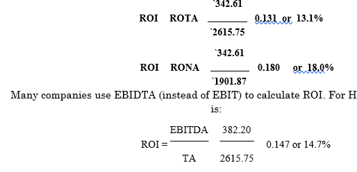
The interest coverage ratio shows the number of times the interest charges are covered by funds that are ordinarily available for their payment. Since taxes are computed after interest, interest coverage is calculated in relation to before-tax earnings. Depreciation is a non-cash item. Therefore, funds equal to depreciation are also available to pay interest charges. We can thus calculate the interest average ratio as earnings before interest taxes, depreciation and amortization (EBITDA) divided by interest:

This ratio indicates the extent to which earnings may fall without causing any embarrassment to the firm regarding the payment of the interest charges. A higher ratio is desirable; but too high a ratio indicates that the firm is very conservative in using debt, and that it is not using credit to the best advantage of shareholders. A lower ratio indicates excessive use of debt or inefficient operations. The firm should make efforts to improve the operating efficiency, or to retire debt to have a comfortable coverage ratio.

The limitation of the interest coverage ratio is that it does not consider repayment of loan. Therefore, a more inclusive ratio—the fixed-charges coverage—is calculated. This ratio is calculated by dividing EBITDA by interest plus principal repayment:

In Equation (18) all variables are on before-tax basis. Since only the after-tax earnings are available to repay principal, the principal repayment is converted to a before-tax basis by dividing it by 1 – tax rate. Depreciation and other non-cash charges are added to the numerator to provide a coverage measure in terms of cash flow rather than earnings. Equation (18) can be extended to include other fixed obligations such as preference dividends and lease rentals. Thus, the fixed-charges coverage ratio will be:

It should be obvious that a high level of debt is a problem for a company only if its future cash flows (earnings being a large component) are uncertain. An analyst, therefore, may analyze the variability of the company’s cash flows (or earnings) over time. This may be done by calculating the standard deviation of yearly changes in cash flows (or earnings) relative to the average level of cash flows (or earnings).

Check Your Concepts

1. What is meant by leverage ratio? What are the types of leverage ratios?

2. How are the following ratios calculated: (a) debt ratio; (b) debt-equity ratio; (c) total liabilities-to total assets ratio?

3. How are coverage ratios calculated? What is its significance?

4. What purpose do leverage ratios serve?

ACTIVITY RATIOS

Funds of creditors and owners are invested in various assets to generate sales and profits. The better the management of assets, the larger the amount of sales. Activity ratios are employed to evaluate the efficiency with which the firm manages and utilizes its assets. These ratios are also called turnover ratios because they indicate the speed with which assets are being converted or turned over into sales. Activity ratios, thus, involve a relationship between sales and assets. A proper balance between sales and assets generally reflects that assets are managed well. Several activity ratios can be calculated to judge the effectiveness of asset utilization.

Inventory Turnover

Inventory turnover indicates the efficiency of the firm in producing and selling its product. It is calculated by dividing the cost of goods sold by the average inventory:

Cost of goods sold

Inventory turnover = (20) Average inventory

The average inventory is the average of opening and closing balances of inventory. In a manufacturing company inventory of finished goods is used to calculate inventory turnover. For HMC, the inventory turnover ratio is:

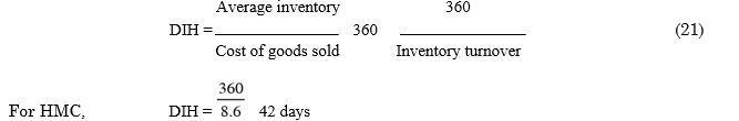
HMC is turning its inventory of finished goods into sales (at cost) 8.6 times in a year. In other words, it holds average inventory of: 12 months/8.6 = 1.4 months, or 360 days/8.6 = 42 days. The reciprocal of inventory turnover gives average inventory holdings in percentage term. When the numbers of days in a year (say, 360) are divided by inventory turnover, we obtain days of inventory holdings (DIH):

The cost of goods sold figure may not be available to an outside analyst from the published annual accounts. He/she may therefore compute inventory turnover as sales divided by the average inventory or the year-end inventory.

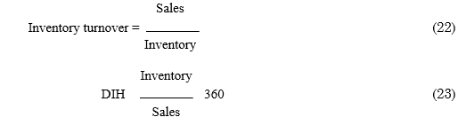
For HMC, the inventory turnover and DIH in terms of sales and year-end inventory are:

`3717.23

It should be noticed that Equation (20) is more logical than Equation (22) in calculating the inventory turnover. In Equation (20) both the numerator—the cost of goods sold and the denominator—the average inventory, are valued at cost and are comparable. While in Equation (22) the numerator—sales—is valued at market price and the denominator is valued at cost and is non-comparable. Further, the average inventory figure is more appropriate to use than the yearend inventory figure because the levels of inventories fluctuate over the year. The average inventory figure smoothes out the fluctuations. If the firm has a strong seasonal character, it is more desirable to take the average of the monthly inventory levels.

Components of inventory The manufacturing firm’s inventory consists of two more components: (i) raw materials and (ii) work-in-process. An analyst may also be interested in examining the efficiency with which the firm converts raw materials into work-in-process and work-in-process into finished goods. That is, the analyst would like to know the levels of raw materials inventory and work in process inventory held by the firm on an average. The raw material inventory should be related to materials consumed, and work-in-process to the cost of production. Thus:

Raw material inventory turnover:

Material consumed can be found out as opening balance of raw material plus purchases minus closing balance of raw material. Cost of production is determined as material consumed plus other manufacturing expenses plus opening balance minus closing balance of work-in-process. In the absence of information of material consumed or cost of production, raw material and work-inprocess inventories may be related to sales.

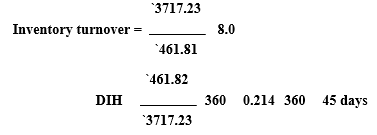
For HMC, the raw material and the work-in-process inventory turnovers are: Raw material inventory turnover

HMC’s inventories of raw material and work-in-process on an average turn, respectively, 6.5 times and 17 times in a year. Interpreted differently, the company holds 55 days’ (i.e., 360/6.5) inventory of raw material and 21 days’ (i.e., 360/17) inventory of work-in-process.

What does inventory turnover indicate? The inventory turnover shows how rapidly the inventory is turning into receivable through sales. Generally, a high inventory turnover is indicative of good inventory management. A low inventory turnover implies excessive inventory levels than warranted by production and sales activities, or a slow-moving or obsolete inventory. A high level of sluggish inventory amounts to unnecessary tie-up of funds, reduced profit and increased costs. If the obsolete inventories have to be written off, this will adversely affect the working capital and liquidity position of the firm. However, a relatively high inventory turnover should be carefully analysed. A high inventory turnover may be the result of a very low level of inventory, which results in frequent stock outs; the firm may be living from hand-to-mouth. The turnover will also be high if the firm replenishes its inventory in too many small lot sizes. The situations of frequent stock outs and too many small inventory replacements are costly for the firm. Thus, too high and too low inventory turnover ratios should be investigated further. The computation of inventory turnovers for individual components of inventory may help to detect the imbalanced investments in the various inventory components.

To judge whether HMC’s inventory turnover is good or not, it should be compared with the past and the expected ratios as well as with inventory turnover ratios of similar firms and industry average. The HMC’s trend in inventory turnover ratios is given in Table 20.6.

Table 20.6: Hindustan Manufacturing Company

Inventory Turnover Ratio

	20X1	20X2	20X3
Finished goods turnover	12.9 (28)	11.9 (30)	8.6 (42)
Work-in-process turnover	27.0 (13)	20.5 (18)	17.1 (21)
Materials turnover	6.5^* (55)	6.4 (56)	6.5 (55)
Sales to total inventory	4.9^** (73)	3.6^**(100)	3.2^**(113)
Inventory to sales	20.4%	27.8%	31.3%

Notes: Numbers within parenthesis give number of days inventory holdings.

* Year-end inventory is used for calculating 20X1 ratio.

** Total of year-end inventory of raw material, work-in-process and finished goods are used.

HMC’s efficiency in turning its inventories is continuously deteriorating. The company’s utilization of inventories in generating sales is poor; the yearly holding of all types of inventories is increasing.

Debtors (Accounts Receivable) Turnover

A firm sells goods for cash and credit. Credit is used as a marketing tool by a number of companies. When the firm extends credits to its customers, debtors (accounts receivables) are created in the firm’s accounts. Debtors are convertible into cash over a short period and, therefore, are included in current assets. The liquidity position of the firm depends on the quality of debtors to a great extent. Financial analysts apply three ratios to judge the quality or liquidity of debtors: (a) debtors turnover, (b) collection period, (c) aging schedule of debtors.

Debtors turnover Debtors turnover is found out by dividing credit sales by average debtors:

Debtors turnover indicates the number of times debtors turnover each year. Generally, the higher the value of debtors turnover, the more efficient is the management of credit.

To an outside analyst, information about credit sales and opening and closing balances of debtors may not be available. Therefore, debtors turnover can be calculated by dividing total sales by the year-end balance of debtors:

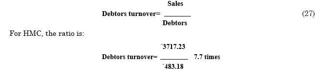
Collection period HMC is able to turnover its debtors 7.7 times in a year. In other words, its debtors remain outstanding for: 12 months/7.7 = 1.56 months or 360 days/7.7 = 47 days. The average number of days for which debtors remain outstanding is called the average collection period (ACP) and can be computed as follows:

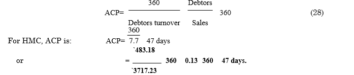
Note that HMC’s debtors are 13 per cent of its sales. For making calculation of ACP, we have used sales for the year. It would be consistent to do so when the firm has constant sales rate throughout the year. ACP calculated on the basis of sales for the year will give a distorted and misleading picture of the firm’s collection rate if sales are seasonal or rapidly growing. ACP calculated at different points of time will vary on account of varying sales rate although there may not be any change in collection rate. Therefore, ACP in the case of seasonal or growing firms should be interpreted cautiously.

What does collection period measure? The average collection period measures the quality of debtors since it indicates the speed of their collection. The shorter the average collection period, the better the quality of debtors, since a short collection period implies the prompt payments by debtors. The average collection period should be compared against the firm’s credit terms and policy to judge its credit and collection efficiency. For example, if the credit period granted by a firm is 35 days, and its average collection period is 50 days, the comparison reveals that the firm’s debtors are outstanding for a longer period than warranted by the credit period of 35 days. An excessively long collection period implies a very liberal and inefficient credit and collection performance. This certainly delays the collection of cash and impairs the firm’s liquidity. The chances of bad debt losses are also increased. On the other hand, a low collection period is not necessarily favourable. Rather, it may indicate a very restrictive credit and collection policy. Because of the fear of bad debt losses, the firm sells only to those customers whose financial conditions are undoubtedly sound, and who are very prompt in making the payment. Such a policy succeeds in avoiding the bad debt losses, but it so severely curtails sales that overall profits are reduced. The firm should consider relaxing its credit and collection policy to enhance the sales level and improve profitability. In addition to measuring the firm’s credit-and-collection efficiency with its own credit terms, the analyst must compare the firm’s average collection period with the industry average. If there is a great divergence between the industry average and the firm’s average collection period, the analyst must investigate the causes. The investigation may reveal that the firm manages its debtors more efficiently or inefficiently than the industry, or its credit policy is too liberal or too restrictive. This may warrant a change in the credit policy. The effect of the changes in the firm’s existing credit policy on sales, profits and liquidity should be analyzed.

The collection period ratio thus helps an analyst in two respects:⁷

in determining the collectibility of debtors and thus, the efficiency of collection efforts, and
in ascertaining the firm’s comparative strength and advantage relative to its credit policy and performance vis-à-vis the competitors’ credit policies and performance.

It is useful to examine the trend in ACP to know the firm’s collection experience. HMC’s debtors turnover, ACP and debtors to sales ratio for three years are given in Table 20.7.

Table 20.7: Hindustan Manufacturing Company

Days of Sales Outstanding

	20X1	20X2	20X3
Debtors turnover (times)	9.2	8.3	7.7
Average collection period (days)	39	43	47
Debtors/sales ratio (per cent)	10.9	12.1	13.0

HMC’s average collection period has been increasing; it has increased from 39 days in 20X1 to 47 days in 20X3. This increase may be due to change in the economic conditions and/or laxity in managing receivables.

Aging schedule The average collection period measures the quality of debtors in an aggregative way. We can have a detailed idea of the quality of debtors through the aging schedule. The aging schedule breaks down debtors according to the length of time for which they have been outstanding. A hypothetical example of the aging schedule is given in Table 20.8.

The aging schedule given in Table 20.8 shows that within the collection period ranging between zero to 25 days, 50 per cent of its debtors are overdue. It also reveals that some of the accounts of the firm have serious problems of collection. The aging schedule gives more information than the collection period, and very clearly spots out the slow-paying debtors.

Table 20.8: Example of Debtors Aging Schedule

Outstanding Period	Outstanding Amount of	Percentage of Total
(days)	Debtors (`)	Debtors
0–25	2,00,000	50.0
26–35	1,00,000	25.0
36–45	50,000	12.5

(Contd…)

Assets Turnover Ratios

Assets are used to generate sales. Therefore, a firm should manage its assets efficiently to maximize sales. The relationship between sales and assets is called assets turnover. Several assets turnover ratios can be calculated.

Net assets turnover The firm can compute net assets turnover simply by dividing sales by net assets (NA).

It may be recalled that net assets (NA) include net fixed assets (NFA) and net current assets (NCA), that is, current assets (CA) minus current liabilities (CL). Since net assets equal capital employed, net assets turnover may also be called capital employed turnover. For Hindustan, the ratio is

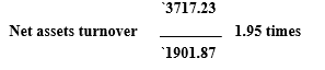
The net assets turnover of 1.95 times implies that Hindustan is producing `1.95 of sales for one rupee of capital employed in net assets.

A firm’s ability to produce a large volume of sales for a given amount of net assets is the most important aspect of its operating performance. Unutilized or under-utilized assets increase the firm’s need for costly financing as well as expenses for maintenance and upkeep. The net assets turnover should be interpreted cautiously. The net assets in the denominator of the ratio include fixed assets net of depreciation. Thus old assets with lower book (depreciated) values may create a misleading impression of high turnover without any improvement in sales.

Some analysts exclude intangible assets like goodwill, patents, etc., while computing the net assets turnover. Similarly, fictitious assets, accumulated losses or deferred expenditures may also be excluded for calculating the net assets turnover ratio.

Total assets turnover Some analysts like to compute the total assets turnover in addition to or instead of the net assets turnover. This ratio shows the firm’s ability in generating sales from all financial resources committed to total assets. Thus:

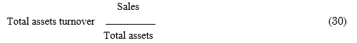
Total assets

Total assets (TA) include net fixed assets (NFA) and current assets (CA) (TA = NFA + CA). For Hindustan, the ratio is:

The total assets turnover of 1.42 times implies that Hindustan generates a sale of `1.42 for one rupee investment in fixed and current assets together.

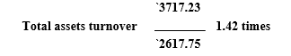
Fixed and current assets turnover The firm may wish to know its efficiency of utilizing fixed assets and current assets separately. For HMC, the fixed assets turnover is:

Sales

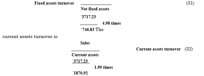
HMC turns over its fixed assets faster than current assets. Interpreting the reciprocals of these ratios, one may say that for generating a sale of one rupee, the company needs, respectively, `0.20 investment in fixed assets and `0.50 investment in current assets.

As explained previously, the use of depreciated value of fixed assets in computing the fixed assets turnover may render comparison of firm’s performance over a period or with other firms meaningless. Therefore, gross fixed assets (GFA) may be used to calculate the fixed assets turnover for a meaningful comparison.

Working capital turnover A firm may also like to relate net current assets (or net working capital gap) to sales. It may thus compute net working capital turnover by dividing sales by net working capital. For HMC, the ratio is:

The reciprocal of the ratios is 0.31. Thus it is indicated that for one rupee of sales, the company needs `0.31 of net current assets. This gap will be met from bank borrowings and long-term sources of funds.

Table 20.9 gives the three-year summary of assets turnover ratios for the HMC’s turnover ratios do not show much improvement. The company has marginally improved its utilization of fixed assets, but its current assets turnover is declining.

Table 20.9: Hindustan Manufacturing Company

Assets Turnover Ratios

	20X1	20X2	20X3
Current assets turnover (sales/CA)	2.70(37.0)	2.01(49.8)	1.99(50.3)
Net current assets turnover (sales/NCA)	3.85(26.0)	3.06(32.7)	3.22(31.1)
Fixed assets turnover (sales/NFA)	4.28(23.4)	4.26(23.5)	4.98(20.1)
Total assets turnover (sales/TA)	1.66(60.4)	1.37(73.2)	1.42(70.4)
Net assets or capital employed turnover (sales/NA)	2.03(49.3)	1.78(56.1)	1.95(51.3)

Note: Numbers in parenthesis represent assets as percentage of sales.

Check Your Concepts

1. What is meant by activity ratio? Why are activity ratios also called turnover ratios? What are thetypes of activity ratios?

2. How are the following ratios calculated: (a) assets turnover ratio; (b) current asset turnover ratio; (c) fixed assets turnover ratio; (d) Net assets turnover ratio; and (e) net current assets turnover ratio?

3. What purpose do activity ratios serve?

PROFITABILITY RATIOS

A company should earn profits to survive and grow over a long period of time. Profits are essential, but it would be wrong to assume that every action initiated by the management of a company should be aimed at maximizing profits, irrespective of concerns for customers, employees, suppliers or social consequences. It is unfortunate that the word ‘profit’ is looked upon as a term of abuse since some firms always want to maximize profits at the cost of employees, customers and society. Except such infrequent cases, it is a fact that sufficient profits must be earned to sustain the operations of the business to be able to obtain funds from investors for expansion and growth and to contribute towards the social overheads for the welfare of the society.⁸

Profit is the difference between revenues and expenses over a period of time (usually one year). Profit is the ultimate ‘output’ of a company, and it will have no future if it fails to make sufficient profits. Therefore, the financial manager should continuously evaluate the efficiency of the company in term of profits. The profitability ratios are calculated to measure the operating efficiency of the company. Besides management of the company, creditors and owners are also interested in the profitability of the firm. Creditors want to get interest and repayment of principal regularly. Owners want to get a required rate of return on their investment. This is possible only when the company earns enough profits.

Generally, two major types of profitability ratios are calculated:

profitability in relation to sales
profitability in relation to investment.

How is Profit Measured?

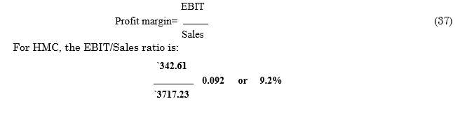
As already discussed in Chapter 2, profit can be measured in various ways. Gross profit (GP) is the difference between sales and the manufacturing cost of goods sold. A number of companies in India define gross profit differently. They define it as earnings profit before depreciation, interest and taxes (PBDIT or EBDIT). A number of multinational companies call this profit or earnings measure as earnings before interest, taxes and depreciation, and amortization or EBITDA. The most common measure of profit is profit after taxes (PAT), or net income (NI), which is a result of the impact of all factors on the firm’s earnings. Taxes are not controllable by management. To separate the influence of taxes, therefore, profit before taxes (PBT) may be computed. If the firm’s profit has to be examined from the point of view of all investors (lenders and owners), the appropriate measure of profit is operating profit. Operating profit is equivalent of earnings before interest and taxes (EBIT). This measure of profit shows earnings arising directly from the commercial operations of the business without the effect of financing. The concept of EBIT may be broadened to include non-operating income if they exist. On an after-tax basis, profit to investors is equal to: EBIT (1 – T), where T is the corporate tax rate. This profit measure is called net operating profit after tax or NOPAT.

Gross Profit Margin

The first profitability ratio in relation to sales is the gross profit margin (or simply gross margin ratio⁹). It is calculated by dividing the gross profit by sales:

Sales Cost of goods sold Gross profit margin

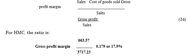
The gross profit margin reflects the efficiency with which management produces each unit of product. This ratio indicates the average spread between the cost of goods sold and the sales revenue. When we subtract the gross profit margin from 100 per cent, we obtain the ratio of cost of goods sold to sales. Both these ratios show profits relative to sales after the deduction of production costs, and indicate the relation between production costs and selling price. A high gross profit margin relative to the industry average implies that the firm is able to produce at relatively lower cost.

A high gross profit margin ratio is a sign of good management. A gross margin ratio may increase due to any of the following factors;¹⁰ (i) higher sales prices, cost of goods sold remaining constant, (ii) lower cost of goods sold, sales prices remaining constant, (iii) a combination of variations in sales prices and costs, the margin widening and (iv) an increase in the proportionate volume of higher margin items. The analysis of these factors will reveal to the management how a depressed gross profit margin can be improved.

A low gross profit margin may reflect higher cost of goods sold due to the firm’s inability to purchase raw materials at favourable terms, inefficient utilization of plant and machinery, or over-investment in plant and machinery, resulting in higher cost of production. The ratio will also be low due to a fall in prices in the market, or marked reduction in selling price by the firm in an attempt to obtain large sales volume, the cost of goods sold remaining unchanged. The financial manager must be able to detect the causes of a falling gross margin and initiate action to improve the situation.

Net Profit Margin

Net profit is obtained when operating expenses, interest and taxes are subtracted from the gross profit. The net profit margin ratio is measured by dividing profit after tax by sales:

` 3717.23

If the non-operating income figure is substantial, it may be excluded from PAT to see profitability arising directly from sales. For HMC, operating profit after taxes to sales ratio is 3.6 per cent.

Net profit margin ratio establishes a relationship between net profit and sales and indicates management’s efficiency in manufacturing, administering and selling the products. This ratio is the overall measure of the firm’s ability to turn each rupee sales into net profit. If the net margin is inadequate, the firm will fail to achieve satisfactory return on shareholders’ funds.

This ratio also indicates the firm’s capacity to withstand adverse economic conditions. A firm with a high net margin ratio would be in an advantageous position to survive in the face of falling selling prices, rising costs of production or declining demand for the product. It would really be difficult for a low net margin firm to withstand these adversities. Similarly, a firm with high net profit margin can make better use of favourable conditions, such as rising selling prices, falling costs of production or increasing demand for the product. Such a firm will be able to accelerate its profits at a faster rate than a firm with a low net profit margin.

An analyst will be able to interpret the firm’s profitability more meaningfully if he/she evaluates both the ratios—gross margin and net margin—jointly. To illustrate, if the gross profit margin has increased over the years, but the net profit margin has either remained constant or declined, or has not increased as fast as the gross margin, it implies that the operating expenses relative to sales have been increasing. The increasing expenses should be identified and controlled. Gross profit margin may decline due to fall in sales price or increase in the cost of production. As a consequence, net profit margin will decline unless operating expenses decrease significantly. The crux of the argument is that both the ratios should be jointly analysed and each item of expense should be thoroughly investigated to find out the causes of decline in any or both the ratios.

Net Margin Based on NOPAT

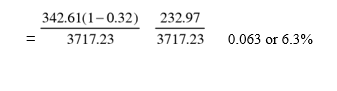
The profit after tax (PAT) figure excludes interest on borrowing. Interest is tax deductible, and therefore, a firm that pays more interest pays less tax. Tax saved on account of payment of interest is called interest tax shield. Thus the conventional measure of net profit margin—PAT to sales ratio—is affected by the firm’s financing policy. It can mislead if we compare two firms with different debt ratios. For a true comparison of the operating performance of firms, we must ignore the effect of financial leverage, viz., the measure of profit should ignore interest and its tax effect. Thus net profit margin (for evaluating operating performance) may be computed in the following way:¹¹

where T is the corporate tax rate. EBIT (1 – T) is the after-tax operating profit, assuming that the firm has no debt.

We can see in Table 20.1 that the effective tax rate for the HMC in 20X3 is 32 per cent. Therefore, the net margin (modified) ratio is:

Taxes are not controllable by a firm, and also, one may not know the marginal corporate tax rate while analysing the published data. Therefore, the margin ratio may be calculated on beforetax basis:12, 13

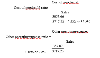
The operating ratio for HMC indicated that 91.8 per cent of sales have been consumed together by the cost of goods sold and other operating expenses. This implies that 8.2 per cent of sales is left to cover interest, taxes, and earnings to owners. Other incomes contribute about 1 per cent of sales. In practice, a firm may decompose the operating expense ratio into: (a) cost of goods sold ratio and (b) other operating expense ratio. For HMC, these ratios are calculated as follows:

What does operating expense ratio reveal? A higher operating expenses ratio is unfavourable since it will leave a small amount of operating income to meet interest, dividends, etc. To get a comprehensive idea of the behaviour of operating expenses, variations in the ratio over a number of years should be studied. Certain expenses are within the managerial discretion; therefore, it should be seen whether change in discretionary expenses is due to changes in the management policy. Detailed analysis may reveal that the year-to-year variations in the operating expense ratio are temporary in nature arising due to some temporary conditions. The variations in the ratio, temporary or long-lived, can occur due to several factors such as: (a) changes in the sales prices, (b) changes in the demand for the product, (c) changes in the administrative or selling expenses or (d) changes in the proportionate shares of sales of different products with varying gross margins. These and other causes of variations in the operating ratio should be thoroughly examined.

The operating expense ratio is a yardstick of operating efficiency, but it should be used cautiously. It is affected by a number of factors, such as external uncontrollable factors, internal factors, employees and managerial efficiency (or inefficiency), all of which are difficult to analyse. Further, the ratio cannot be used as a test of financial condition in the case of those firms where nonoperating revenue and expenses form a substantial part of the total income.

The operating expense ratio indicates the average aggregative variations in expenses, where some of the expenses may be increasing while others may be falling. Thus, to know the behaviour of specific expense items, the ratio of each individual operating expense to sales should be calculated. These ratios when compared from year to year for the firm will throw light on managerial policies and programmes. For example, the increasing selling expenses, without a sufficient increase in sales, can imply uncontrolled sales promotional expenditure, inefficiency of the marketing department, general rise in selling expenses or introduction of better substitutes by competitors. The expenses ratios of the firm should be compared with the ratios of the similar firms and the industry average. This will reveal whether the firm is paying higher or lower salaries to its employees as compared to other firms; whether its capacity utilization is high or low; whether the salesmen are given enough commission; whether it is unnecessarily spending on advertisement and other sales promotional activities; whether its cost of production is high or low and so on.

Return on Investment (ROI)

The term investment may refer to total assets or net assets. The funds employed in net assets is known as capital employed. Net assets equal net fixed assets plus current assets minus current liabilities excluding bank loans. Alternatively, capital employed is equal to net worth plus total debt.

The conventional approach of calculating return on investment (ROI) is to divide PAT by investment. Investment represents pool of funds supplied by shareholders and lenders, while PAT represents residue income of shareholders; therefore, it is conceptually unsound to use PAT in the calculation of ROI. Also, as discussed earlier, PAT is affected by capital structure. It is therefore more appropriate to use one of the following measures of ROI for comparing the operating efficiency of firms:

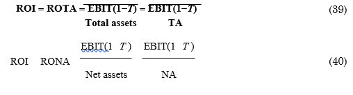
where ROTA and RONA are, respectively, return on total assets and return on net assets. RONA is equivalent of return on capital employed, i.e., ROCE. The after tax ROTA and RONA for HMC are

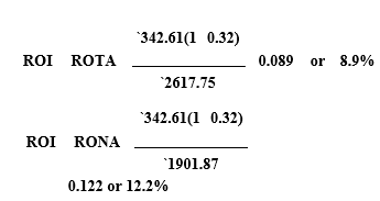
 0.122 or 12.2%

Since taxes are not controllable by management, and since firm’s opportunities for availing tax incentives differ, it may be more prudent to use before-tax measure of ROI. Thus, the beforetax ratios are:¹⁴

EBIT

ROI/ROTA (41)

EBIT

ROI /RONA (42)

For HMC, the before-tax ROI is:

Return on Equity (ROE)

Common or ordinary shareholders are entitled to the residual profits. The rate of dividend is not fixed; the earnings may be distributed to shareholders or retained in the business. Nevertheless, the net profits after taxes represent their return. A return on shareholders’ equity is calculated to see the profitability of owners’ investment. The shareholders’ equity or net worth will include paid-up share capital, share premium and reserves and surplus less accumulated losses. Net worth can also be found by subtracting total liabilities from total assets.

The return on equity is net profit after taxes divided by shareholders’ equity which is given by net worth:¹⁵

ROE indicates how well the firm has used the resources of owners. In fact, this ratio is one of the most important relationships in financial analysis. The earning of a satisfactory return is the most desirable objective of a business. The ratio of net profit to owners’ equity reflects the extent to which this objective has been accomplished. This ratio is, thus, of great interest to the present as well as the prospective shareholders and also of great concern to the management, which has the responsibility of maximizing the owners’ welfare.

The returns on owners’ equity of the company should be compared with the ratios for other similar companies and the industry average. This will reveal the relative performance and strength of the company in attracting future investments.

The trend in sales and assets-based profitability ratios for HMC is given below:

Table 20.10: Hindustan Manufacturing Company

Profitability Ratios

	20X1	20X2	20X3
Gross Margin	0.175	0.178	0.179
Net Margin	0.036	0.039	0.036
EBIT/Sales	0.079	0.094	0.092
PAT/Total Assets	0.059	0.054	0.052
EBIT/Total Assets	0.131	0.129	0.131
PAT/Net Assets	0.072	0.070	0.071
EBIT/Net Assets	0.161	0.168	0.180
Return on Equity	0.164	0.191	0.200

It can be seen from Table 20.10 that sales as well as investment related ratios of the company have remained more or less constant. Return on equity has shown an increase. This is perhaps due to the use of more debt over years by the company.

Check Your Concepts

1. What is meant by profitability ratio? What are the types of profitability ratios?

2. What are sales-related profitability ratios? How are they calculated?

3. How do you calculate EBIT, NOPAT and EBITDA? How do they relate to sales and assets?

4. How will you define ‘investment’ to measure investment-related profitability ratio?

5. Is it appropriate to calculate PAT-to-total or net assets ratio? Why or why not?

6. Briefly explain the significance of profitability ratios?

Earnings per Share (EPS)

The profitability of the shareholders’ investment can also be measured in many other ways. One such measure is to calculate the earnings per share. The earnings per share (EPS) is calculated by dividing the profit after taxes by the total number of ordinary shares outstanding.

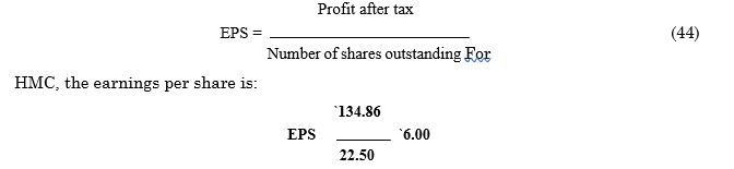
EPS calculations made over the years indicate whether or not the firm’s earnings power on per-share basis has changed over that period. The EPS of the company should be compared with the industry average and the earnings per share of other firms. EPS simply shows the profitability of the firm on a per-share basis; it does not reflect how much is paid as dividend and how much is retained in the business. But as a profitability index, it is a valuable and widely used ratio.

Bonus and rights issues adjustment Adjustments for bonus or rights issues should be made while comparing EPS over a period of time. Bonus shares are free additional shares issued (through a transfer from reserves and surplus to the share capital) to the shareholders. The total wealth of a shareholder before or after bonus issue remains the same. Suppose the share price before bonus issue is `100, and a bonus issue of 1:3 is made. A shareholder holding 3 shares before bonus issue has a wealth of: `100 × 3 = `300. Since no cash flow takes place when bonus shares are issued his/her total wealth remains the same but is now divided into 4 shares. Thus, the share price after bonus is diluted to: `300/4 = `75 (ex-bonus price).

For a proper comparison of EPS, DPS (dividend per share), book value and share price for the periods before bonus issue, the data for the periods after bonus issue should be adjusted. For example, if a bonus issue in the proportion of 1:3 is made, then the adjustment factor 4/3 should be applied to adjust EPS of the year in which bonus issue is made as well as the subsequent years. Further, if the bonus issue, say, of 1:5 is made once again after some years, then the adjustment factor will become: 4/3 × 6/5 = 24/15 = 1.68, for the bonus year and subsequent years.

Rights issues are the shares issued to the existing shareholders of a company at a subscription price that may be different (generally lower) from the current share price. Suppose the market price of a company’s share is `100, and the subscription price per share under a rights issue is `60. The share price of `100 with the rights is called cum-rights price. Further, assume that 3 rights are needed to subscribe to one share (i.e., 1:3 rights issue). What is the implication of this for the shareholder’s wealth? Before the rights issue, the wealth of the shareholder holding 3 shares is: `100 × 3 = `300. After subscribing to the rights issue, he/she owns one additional share by paying `60. Thus, the shareholder now has a wealth of: `300 + `60 = `360 divided into 4 shares. Thus, the price per share after exercising the rights (ex-rights price) will be: `360/4 = `90. The shareholder’s existing wealth remains unchanged; he/she has paid `60 to increase his/her wealth by this amount. However, the shareholder’s proportionate ownership remains the same when he/she exercises the rights. When the rights shares have been issued, EPS, DPS, book value and share price are diluted (as the number of shares increase). To make them comparable with the data of earlier periods (before the issue of rights), they should be adjusted for the effect of the rights issue. In the example, the rights adjustment factor will be in proportion to cum-right and ex-right prices: 100/90 = 1.11.

Dividend per Share (DPS or DIV)

The net profits after taxes belong to shareholders. But the income, which they really receive, is the amount of earnings distributed as cash dividends. Therefore, a large number of present and potential investors may be interested in DPS, rather than EPS. DPS is the earnings distributed to ordinary shareholders divided by the number of ordinary shares outstanding:

The company distributed `2.00 per share as dividend out of `6.00 earned per share. The difference per share is retained in the business. Like in the case of EPS, adjustments for bonus or rights issues should be made while calculating DPS over the years.

Dividend-Payout Ratio

The dividend-payout ratio or simply payout ratio is DPS (or total equity dividends) divided by the EPS (or profit after tax):

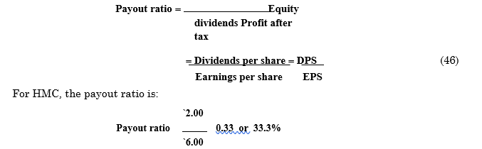
`6.00

Earnings not distributed to shareholders are retained in the business. Thus retention ratio is: 1 – Payout ratio. If this figure is multiplied by the return on equity (ROE), we can know the growth in the owners’ equity as a result of retention policy. Thus, HMC, the growth in equity is:¹⁶

Growth in equity = Retention ratio × ROE

g = b × ROE (47)

For HMC, growth in equity is as follows:

g= 0.667 ¥ 0.20 = 0.133 or 13.3%

Dividend Yield and Earnings Yield

The dividend yield is the dividends per share divided by the market value per share, and the earnings yield is the earnings per share divided by the market value per share. That is:

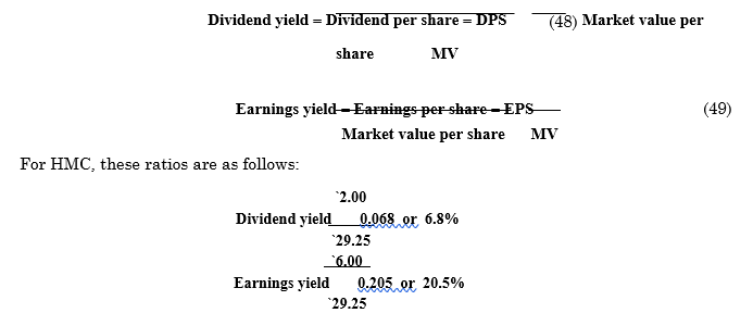
The dividend yield and earnings yield evaluate the shareholders’ return in relation to the market value of the share. The earnings yield is also called the earnings–price (E/P) ratio. The information on the market value per share is not generally available from the financial statements; it has to be collected from external sources, such as the stock exchanges or the financial newspapers.

Price–Earnings Ratio

The reciprocal of the earnings yield is called the price–earnings (P/E) ratio. Thus:

The price-earnings ratio is widely used by the security analysts to value the firm’s performance as expected by investors. It indicates investors’ judgement or expectations about the firm’s performance. Management is also interested in this market appraisal of the firm’s performance and will like to find the causes if the P/E ratio declines.

P/E ratio reflects investors’ expectations about the growth in the firm’s earnings. Industries differ in their growth prospects; accordingly, the P/E ratios for industries vary widely.

Market Value-to-Book Value (MV/BV) Ratio

Market value-to-book value (M/B) ratio is the ratio of share price to book value per share

HMC:

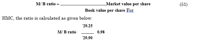
Note that book value per share is net worth divided by the number of shares outstanding. HMC’s M/B ratio of 0.98 means that the company is worth 2 per cent less than the funds, which shareholders have put into it.

Tobin’s q

Tobin’s q is the ratio of the market value of a firm’s assets (or equity and debt) to its assets’ replacement costs. Thus

This ratio differs from the market value-to-book value ratio in two respects: it includes both debt and equity in the numerator, and all assets in the denominator, not just the book value of equity. It is argued that firms will have the incentive to invest when q is greater than 1. They will be reluctant to invest once q becomes equal to 1.¹⁷

Table 20.11 gives trend in the company’s EPS, DPS and Market-related profitability ratios.

Table 20.11: Hindustan Manufacturing Company

EPS, DPS and Market-related

Profitability Ratios (` lakh)

	20X1	20X2	20X3
EPS (`)	3.72	4.94	5.99
DPS (`)	1.50	1.75	2.00
Market value (average) (`)	26.38	34.50	29.25
Book value (`)	22.72	25.91	29.90
Dividend payout	0.40	0.35	0.33
Earnings yield	0.141	0.143	0.205
Dividend yield	0.057	0.051	0.068
P/E Ratio (times)	7.09	7.00	4.88
M/B ratio (times)	1.16	1.33	0.98

It is indicated that the company’s EPS and DPS are increasing; but the proportionate increase in DPS is less than that in EPS and therefore dividend payout ratio is declining. EPS may be increasing more as a result of increasing use of debt than due to improved operations. Because of increase in the financial risk, the market price of share may come down. In spite of the increase in EPS and DPS, the market price of Hindustan’s share has declined to `29.25 in 20X3. As a result, the P/E ratio has substantially reduced to 4.88 in 20X3. The market value-to-book value ratio has also declined to 0.98. Thus, in terms of market performance, the company is showing deterioration.

Check Your Concepts

1. What ratios are shareholders interested in?

2. How are the following ratios calculated: (a) EPS; (b) DPS; (c) market-to-book value; (d) book value per share?

3. How and why are price-earnings ratio, earnings yield and dividend yield calculated?

4. How do bonus shares and rights issues affect EPS and DPS? What adjustment is needed to be madeto compare EPS and DPS across time?

EVALUATION OF A FIRM’S EARNING POWER: DUPONT ANALYSIS

RONA (or ROCE) is the measure of the firm’s operating performance. It indicates the firm’s earning power. It is a product of the asset turnover, gross profit margin and operating leverage.¹⁸Thus, RONA can be computed as follows:

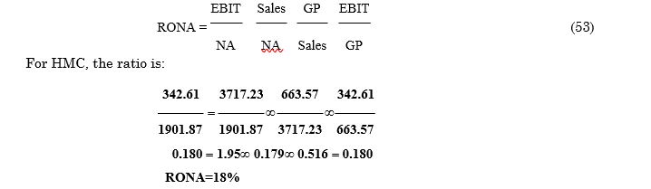
It may be seen from Table 20.12 that HMC’s RONA has shown improvement over the years in spite of a constant gross margin and slightly declining assets turnover. RONA has increased on account of a higher operating leverage, as measured by EBIT/GP ratio, employed by the company.

All firms would like to improve their RONA. In practice, however, competition puts a limit on RONA. Also, firms may have to trade-off between asset turnover and gross profit margin. To improve profit margin, some firms resort to vertical integration for cost reduction and synergistic benefits.

A firm can convert its RONA into an impressive ROE through financial efficiency. Financial leverage and debt-equity ratios affect ROE and reflect financial efficiency. ROE is thus a product of RONA (reflecting operating efficiency) and financial leverage ratios (reflecting financing efficiency):

For HMC, the ratio is:

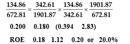
HMC’s PAT/EBIT has deteriorated, while the net assets/equity (NA/NW) ratio has increased over a period. The combined effect (1.12), however, has been favourable; Hindustan’s ROE has increased to 20.0 per cent. The product of PAT/EBIT and NA/NW is referred to as the leverage factor.

A firm can convert its ROE into growth in equity through retention. Equity growth as a result of retention policy is a product of ROE and retention ratio:

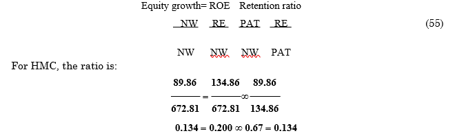
HMC’s retention ratio has increased over the years. With an increasing ROE this has resulted in higher growth in equity over the years.

The combined effect of three aspects—operating efficiency, financing efficiency and retention— shows that HMC has a steadily improving performance (Table 20.12). The computations of ratios in Table 20.12 clearly show the interaction between operating (turnover) ratios, profitability ratios and leverage ratios for obtaining return on the shareholders’ earnings. Thus:

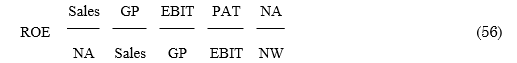
As shown earlier, ROE multiplied by retention ratio gives growth. A chart (sometimes known as a DuPont chart) can also be used to depict HMC’s performance in terms of shareholders’ return (see Figure 20.1).

Table 20.12: Hindustan Manufacturing Company

Analysis of Earning Power (` lakh)

			20X1	20X2	20X3
	A. Sales/NA	Turnover	2.03	1.78	1.95
	B. GP/Sales	Gross margin	0.175	0.178	0.179
	C. EBIT/GP	Operating leverage	0.452	0.529	0.516
	D. EBIT/NA (A × B × C)	RONA	0.161	0.168	0.180
	E. PAT/EBIT	Financial leverage	0.452	0.418	0.394
	F. NA/NW	Financial leverage	2.26	2.72	2.83
	G. PAT/NW (D × E × F)	ROE	0.164	0.191	0.200
	H. RE/PAT	Retention	0.60	0.65	0.67
	I. RE/NW (G × H)	Equity growth	0.098	0.123	0.134
*Check Your Concepts* 1. What is meant by ‘earnings power’? 2. What is DuPont analysis? How does DuPont analysis help in determining a firm’s earnings power? 3. How is ROE determined by the firm’s operating performance and financial leverage? 4. How is growth in equity determined?

COMPARATIVE STATEMENTS ANALYSIS

A simple method of tracing periodic changes in the financial performance of a company is to prepare comparative statements. Comparative financial statements will contain items at least for two periods. Changes—increases and decreases—in income statement and balance sheet over a period can be shown in two ways: (1) aggregate changes and (2) proportional changes.

Drawing special columns for aggregate amount or percentage, or both, of increases and decreases, can indicate aggregate changes. Recording percentage calculated in relation to a common base in special columns, on the other hand, shows relative or proportional changes. For example, in the case of profit and loss statement, sales figure is assumed to be a common base (and therefore, equal to 100) and all other items are expressed as percentage of sales. Similarly, the balance sheet items are expressed as percentage of total assets or total funds. The financial statements prepared in terms of common base percentages are called common-size statements. This kind of analysis is called vertical analysis and it indicates static relationships since relative changes are studied at a specific date.

Table 20.13 shows comparative balance sheets and corresponding changes in balance sheet data for the Hindustan Manufacturing Company.

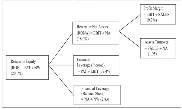
Figure 20.1: DuPont Chart: Hindustan Manufacturing Company’s Financial Performance, 20X3

Table 20.13: Hindustan Manufacturing Company

Comparative Balance Sheet

	(` lakh) 20X2 20X3 Change Per cent Change
Liabilities and Capital Current liabilities	1,123.57 1,555.74(+) 432.17(+) 38.5%
Long-term liabilities	361.65 389.19(+) 27.54(+) 7.6%
Share capital	225.00 225.00 0 0
Reserves	357.95 447.81(+) 89.86(+) 25.1%
Total	2,068.17 2,617.74(+) 549.57(+) 26.6%
Assets Current assets	1,404.55 1,870.92(+) 466.37(+) 33.2%
Net fixed assets	647.18 686.11(+) 38.93(+) 6.0%
Other assets	16.44 60.72(+) 44.28(+) 269.3%
Total	2,068.17 2,617.75(+) 549.58(+) 26.6%

An investigation of the comparative financial statements helps to highlight the significant facts and points out the items which need further analysis. The published balance sheets and profit and loss accounts of joint-stock companies in India are presented in a two-year comparative form. Some of the companies also report to shareholders condensed comparative statements covering an extended period of years. From analytical point of view, such statements are quite useful to investors.

For HMC, the common-size statements are given in Tables 20.14 and 20.15.

Table 20.14: Hindustan Manufacturing Company

Common-size Profit and Loss Statement (` lakh)

20X1 20X2 20X3

Net Sales 100.0 100.0 100.0

17.5	17.8	17.9
10.2	9.3	9.6
7.3	8.5	8.3
0.7	0.9	1.0
8.0	9.4	9.3
2.6	4.4	3.9
5.4	5.0	5.4
1.8	1.1	1.7

Cost of goods sold 82.5 82.2 82.1

Gross profit

Less: Selling and administrative expenses

Operating income

Add: Other income

EBIT

Less: Interest

PBT

Taxes

PAT 3.6 3.9 3.7

Table 20.15: Hindustan Manufacturing Company

Common-size Balance Sheet (` lakh)

		20X1 20X2 20X3
	Current Liabilities Bank borrowing	31.4 31.0 32.1
	Trade creditors	2.5 10.2 13.0
	Provision, etc.	15.8 13.1 14.3
	Total
	Long-term Liabilities Debentures	0.0 3.7 2.9
	Others	14.1 13.8 12.0
	Total
	Total Liabilities	63.8 71.8 74.3
	Net Worth Share capital	15.9 10.9 8.6
	Reserve	20.3 17.3 17.1
	Total
	Total Funds	100.0 100.0 100.0
	Current Assets Cash and bank balance	0.6 4.8 1.0
	Trade debtors	17.9 16.5 18.5
	Inventory: Raw material	17.2 18.5 17.5
	Work-in-process	6.1 7.3 8.8
	Finished goods	10.4 11.8 17.6
	Others	9.1 9.0 8.1
	Total	61.3 67.9 71.5
	Fixed Assets Gross block	46.3 40.7 35.2
	Less: Accumulated dep.	11.3 9.4 9.0
	Net block	35.0 31.3 26.2
	Other non-current assets	3.7 0.8 2.3
	Total	38.7 32.1 28.5
	Total Assets	100.0 100.0 100.0
*Check Your Concepts* 1. What is comparative financial statement analysis? Why is it needed? 2. How is comparative financial statement analysis carried out?

TREND ANALYSIS

In financial analysis the direction of changes over a period of years is of crucial importance. Time series or trend analysis of ratios indicates the direction of change. This kind of analysis is particularly applicable to the items of profit and loss account. It is advisable that trends of sales and net income may be studied in the light of two factors: the rate of fixed expansion or secular trend in the growth of the business and the general price level. It might be found in practice that a number of firms would show a persistent growth over a period of years. But to get a true trend of growth, the sales figures should be adjusted by a suitable index of general prices. In other words, sales figures should be deflated for rising price level. When the resulting figures are shown on a graph, we will get trend of growth devoid of price changes. Another method of securing trend of growth and one which can be used instead of the adjusted sales figures or as a check on them is to tabulate and plot the output or physical volume of sales expressed in suitable units of measure. If the general price level is not considered while analysing trend of growth, it can mislead the management. They may become unduly optimistic in periods of prosperity and pessimistic in dull periods.

For trend analysis, the use of index numbers is generally advocated. The procedure followed is to assign the number 100 to items of the base year and to calculate percentage changes in each items of other years in relation to the base year. This procedure may be called as “trend-percentage method.”

Table 20.16: Hindustan Manufacturing Company

Trend Analysis

	20X1	20X2	20X3
Sales	100	120.8	158.9
EBIT	100	143.6	184.8
PAT	100	132.8	161.0
Current assets	100	162.2	216.0
Current liabilities	100	160.1	221.7
Gross fixed assets	100	128.8	141.0
Net assets	100	137.5	164.8
Total assets	100	146.4	185.3
Net worth	100	114.0	131.6
Dividend	100	116.7	133.3

Table 20.16 gives trend percentages for profit and loss statement and balance sheet items. Hindustan’s EBIT has increased faster than the growth in sales, while PAT has shown slightly better performance than sales. Current assets and current liabilities have moved together. Total assets have grown faster than net worth, which implies greater reliance on outsiders’ money by

HMC.

INTER-FIRM ANALYSIS

A firm would like to know its financial standing vis-à-vis its major competitors and the industry group. As explained earlier, the analysis of the financial performance of all firms in an industry and their comparison at a given point of time is referred to the cross-section analysis or the inter-firm analysis. To ascertain the relative financial standing of a firm, its financial ratios are compared either with its immediate competitors or with the industry average. We have used the data of construction firms to illustrate the inter-firm comparison.

Table 20.17 contains the financial data of eleven construction firms. Table 20.18 shows six important ratios for each firm. These ratios are also shown in Figures 20.2 to 20.7.

CE = capital employed; NW = net worth; NS = net sales; PBIT = profit before interest and tax; PBT = profit before-tax; PAT = profit after-tax; DIV = dividend

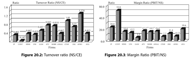
Figure 20.3 shows the proportionate market share of the eleven companies. In terms of the market share, Jaiprakash is the largest company, holding 44 per cent market share, followed by Hindustan Construction with 11 per cent and ATV Projects with 9 per cent. The market shares of next three companies range between 6 and 8 per cent. The last three companies’ market shares vary between 1 and 3 per cent.

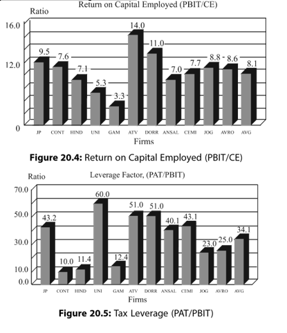
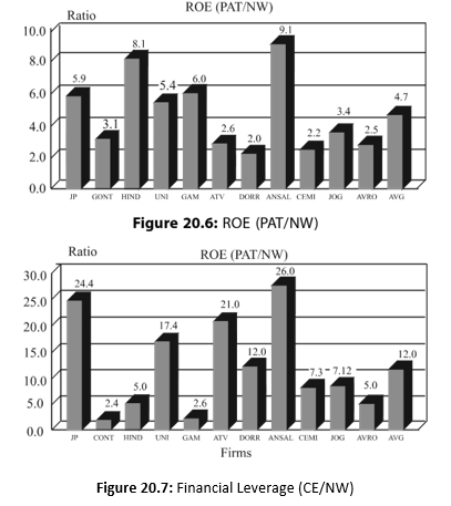
Table 20.17: Financial Data for Construction Companies

Company Name	CE	NW	NS PBIT	PBT		PAT	DIV
Jaiprakash	89,801	15,614	36,139	8,825	3,812	3,812	1,050
Continental	36,601	11,850	5,203	2,791	419	279	330
Hind. Const.	19,779	2,450	9,134	1,410	161	161	113
Unitech	14,264	2,662	5,880	762	639	464	173
Gammon	10,498	1,553	6,383	348	59	43	43
ATV Projects	8,818	3,173	7,433	1,287	702	667	183
Dorroliver	5,683	2,809	4,648	674	648	350	143
Ansal Housing	5,445	598	2,625	431	261	173	236
Cemindia	2,252	1,024	2,264	174	140	75	38
V.M. Jog	1,843	539	1,419	162	60	38	24
Acrow Total (annualized)	781	309	1,073	67	25	18	10
Acrow Total (annualized)	2,03,861	43,658	84,212	16,519	6,482	5,636	2,305

CE = capital employed; NW = net worth; NS = net sales; PBIT = profit before interest and tax; PBT = profit before-tax; PAT = profit after-tax; DIV = dividend.

Figures 20.2 to 20.7 show the relative position of companies regarding various financial dimensions. The industry shows significant variation across firms in terms of all ratios. Although Jaiprakash is the largest company, it is Ansal which has the highest ROE of 28.9 per cent;

Jaiprakash comes at the second place with ROE of 24.4 per cent. Both companies’ ROE is almost

Jaiprakash 44%

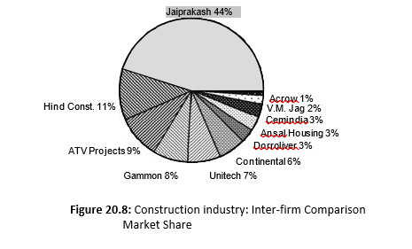
double the industry average. Other ratios can also be interpreted in a similar way.

The top three performers in terms of market share, return on investment and return on equity are as follows.

1. Market share

1. Jaiprakash (44%)

2. Hind. Const. (11%)

3. ATV Projects (9%)

2. ROI: PBIT/CE

1. ATV Projects (14.6%)

2. Dorroliver (11.9%)

3. Jaiprakash (9.8%)

3. ROE: PAT/NW

1. Ansal (28.9%)

2. Jaiprakash (24.4%)

3. ATV Projects (21.0%)

It is notable that the performance of both ATV Projects and Jaiprakash has been consistent. ATV Projects figures in top three firms for almost all ratios. It has highest ROI in the industry, but, because of a low leverage ratio, its ROE is lower than Jaiprakash and Ansal, both highly geared companies. Jaiprakash has highest market share, but low ROI because of the poor utilization of assets in turning over sales. Ansal has been able to obtain highest ROE because of the highest gearing (CE/NW = 1 + debt-equity) of 9.11 in the industry.

Check Your Concepts

1. How and why is trend analysis of ratios performed?

2. Explain the significance of inter-firm comparison?

UTILITY AND LIMITATIONS OF RATIO ANALYSIS

The ratio analysis is the most powerful tool of the financial analysis. As stated in the beginning of the chapter, many diverse groups of people are interested in analyzing the financial information to indicate the operating and financial efficiency, and growth of the firm. These people use ratios to determine those financial characteristics of the firm in which they are interested. With the help of ratios, one can determine:

the ability of the firm to meet its current obligations;
the extent to which the firm has used its long-term solvency by borrowing funds; l the efficiency with which the firm is utilizing its assets in generating sales revenue l the overall operating efficiency and performance of the firm.

Performance analysis As stated previously, a short-term creditor will be interested in the current financial position of the firm, while a long-term creditor will pay more attention to the solvency of the firm. The long-term creditor will also be interested in the profitability of the firm. The equity shareholders are generally concerned with their return and may bother about the firm’s financial condition only when their earnings are depressed. In fact, it has to be realized that the short- and long-term financial position and the profitability of the firm are tested in every kind of financial analysis, but the emphasis would differ. Some ratios are more important in one kind of analysis than others. If a short-term creditor analyses only the current position and finds it satisfactory, he/she cannot be certain about the safety of his/her claim if the firm’s long-term financial position or profitability is unfavourable. The satisfactory current position would become adverse in future if the current resources are consumed by the unfavourable long-term financial condition. Similarly, the ‘good’ long-term financial position is no guarantee for the long-term creditors’ claims if the current position or the profitability of the firm is ‘bad.’

Table 20.18: Financial Ratios for Construction Companies

Company NS/ PBIT/ PBIT/ PAT/ CE/ PAT/

Name CE NS CE PBIT NW NW

Jaiprakash 0.48 24.42% 9.83% 43.20% 5.75 24.41% Continental 0.41 53.64% 7.63% 10.00% 3.09 2.35% Hind. Const. 0.46 15.44% 7.13% 11.42% 8.07 6.57% Unitech 0.41 12.96% 5.34% 60.89% 5.36 17.43%

Gammon 0.61 5.45% 3.31% 12.36% 6.76 2.77%

ATV Projects 0.84 17.31% 14.60% 51.83% 2.78 21.02% Dorroliver 0.82 14.50% 11.86% 51.93% 2.02 12.46% Ansal Housing 0.48 16.42% 7.92% 40.14% 9.11 28.93% Cemindia 1.01 7.69% 7.73% 43.10% 2.20 7.32% V.M. Jog 0.77 11.42% 8.79% 23.46% 3.42 7.05% Acrow 1.37 6.24% 8.58% 26.87% 2.53 5.83%

Wgt. average 0.41 19.62% 8.01% 34.12% 4.67 12.91%

Credit analysis In credit analysis, the analyst will usually select a few important ratios. He may use the current ratio or quick-asset ratio to judge the firm’s liquidity or debt-paying ability or debt-equity ratio to determine the stake of the owners in the business and the firm’s capacity to survive in the long run and any one of the profitability ratios, for example, return on capital employed, to determine the firm’s earnings prospects. If the profitability is high, the current ratio is low and the debt equity ratio is high (unreasonable), the extension of credit may be approved to the firm, because a profitable company will grow and will have improvement in its current ratio and other ratios.

Security analysis The ratio analysis is also useful in security analysis. The major focus in security analysis is on the long-term profitability. Profitability is dependent on a number of factors and, therefore, the security analyst also analyses other ratios. He would certainly be concerned with the efficiency with which the firm utilizes its assets and the financial risk to which the firm is exposed. Therefore, besides analyzing the profitability ratios meticulously, he will also analyze activity ratios and leverage ratios. The detailed analysis of the earning power is important for security analysis.

Competitive analysis The ratios of a firm by themselves do not reveal anything. For meaningful interpretation, the ratios of a firm should be compared with the ratios of similar firms and industry. This comparison will reveal whether the firm is significantly out of line with its competitors. If it is significantly out of line, the firm should undertake a detailed analysis to spot out the trouble areas.

Trend analysis The ratio analysis will reveal the financial condition of the firm more reliably when trends in ratios over time are analysed. Ratios at a point of time can mislead the analyst, because they may be high or low for some exceptional circumstances at that point of time. An impressive present financial position may really be eroding over time, while a weak position may be improving at a rapid rate over time. Thus, the trend analysis of the ratios adds considerable significance to the financial analysis because it studies ratios of several years and isolates the exceptional instances occurring in one or two periods. Although the trend analysis of the company’s ratios itself is informative, it is more informative to compare the trends in the company’s ratios with the trends in industry ratios. This comparison indicates how well the company has been operating over time relative to its competitors and may also help to explain the trends in the company’s ratios. For example, if the company’s return on capital employed (net assets) shows a declining trend, the comparison can reveal whether this decline is characteristic of the firm only or there is a general declining trend in the industry.

The management has to protect the interests of all concerned parties, creditors, owners and others. They have to ensure some minimum operating efficiency and keep the risk of the firm at a minimum level. Their survival depends upon their operating performance. From time to time, the management uses ratio analysis to determine the firm’s financial strengths and weaknesses, and accordingly takes actions to improve the firm’s position. Management is in a better position to analyse the firm’s financial position as it has access to internal information, which is not available to the credit analyst or the security analyst.

Diagnostic Role of Ratios

The essence of the financial soundness of a company lies in balancing its goals, commercial strategy, product-market choices and resultant financial needs. The company should have the financial capability and flexibility to pursue its commercial strategy. Ratio analysis is a very useful analytical technique to raise pertinent questions on a number of managerial issues. It provides bases or clues to investigate such issues in detail. While assessing the financial health of the company with the help of ratio analysis, answers to the following questions relating to the company’s profitability, assets utilization, liquidity, financing and strategies capabilities may be sought:¹⁹

Profitability analysis

How profitable is the company? What accounting policies and practices are followed by thecompany? Are they stable?
Is the profitability (RONA) of the company high/low/average? Is it due to:
- profit margin
- assets utilization
- non-operating income
- window dressing l change in accounting policy l inflationary conditions?
Is the return on equity (ROE) high/low/average? Is it due to:
- return on investment
- financing mix
- capitalization of reserves?
What is the trend in profitability? Is it improving because of better utilization of resourcesor curtailment of expenses of strategic importance? What is the impact of cyclical factors on profitability trend?
Can the company sustain its impressive profitability or improve its profitability given thecompetitive and other environmental situations?

Assets utilization

How effectively does a company utilize its assets in generating sales?
Are the levels of debtors and inventories relative to sales reasonable, given the firm’scompetitive and operating characteristics?
What are the trends in collection period, inventory turnover and fixed assets turnover?
Is the improvement in the fixed assets turnover due to:
- depreciated book value of fixed assets?
- sale of some fixed assets?

Liquidity analysis

What is the level of current assets relative to current liabilities? Is it reasonable given thenature of the company’s business?
What is the mix of current assets? Is the proportion of slow moving inventories high?
How promptly does the company pay its creditors?
How far can it stretch payment to creditors without jeopardizing its relations with them?
How efficiently and frequently does the company convert its current assets into cash?
Given the company’s riskiness and future financial needs, how soundly is it financed?l What is the mix of debt and equity?
- What is the maturity structure of debt? Is the company faced with large debt repayments in the near future?
- Does the company generate enough cash lows to service debt adequately?
- Is the company close to its borrowing limits of restrictive convenants?
Does the company have lease commitments not disclosed in the balance sheet?
Does it have large contingent liabilities?
What potential does the company have to raise debt on acceptable terms? From whom? Onwhat conditions? How quickly?
Can the company raise equity funds? Would market respond favourably? To whom and atwhat price shares would be sold? Is the management willing for dilution of control if shares are issued?

Strategic analysis A number of other questions go beyond the scope of ratio analysis. They however need to be answered while assessing the financial health of the company. These questions are:²⁰

What are the goals and strategies of the company?
How successfully has the company pursued its goals and strategies? Is change in themwarranted?
Are the company’s goals, strategies, product-market choices, investment requirements,financing needs and financing capabilities in balance?
What would happen to the above-referred balance if the company has to face an adversity?
If the company is struck by adversity:
- What kinds of competitive, operating and environmental risks would occur?
- How would management respond in strategic and operating terms?
- What kinds of financial pressures would be faced?
- Would it be able to raise necessary funds on acceptable terms?
- Would the company be able to use its reserve resources? In what sequence would these resources be used?

CAUTIONS IN USING RATIO ANALYSIS

The ratio analysis is a widely used technique to evaluate the financial position and performance of a business. But there are certain problems in using ratios. The analyst should be aware of these problems. The following are some of the limitations of the ratio analysis:²¹

It is difficult to decide on the proper basis of comparison.
The comparison is rendered difficult because of differences in situations of two companies or of one company over the years.
The price level changes make the interpretations of ratios invalid.
The differences in the definitions of items in the balance sheet and the profit and loss statement make the interpretation of ratios difficult.
The ratios calculated at a point of time are less informative and defective as they suffer from short-term changes.
The ratios are generally calculated from past financial statements and, thus are no indicators of future.

Standards for comparison Ratios of a company have meaning only when they are compared with some standards. It is difficult to find out a proper basis of comparison. Usually, it is recommended that ratios should be compared with industry averages. But the industry averages are not easily available. In India, industry data on financial ratios are available from company finance studies conducted by the Reserve Bank of India. CMIE (Center for Monitoring Indian Economy) provides large database of companies as well as ratios.

Company differences Situations of two companies are never same. Similarly, the factors influencing the performance of a company in one year may change in another year. Thus, the comparison of the ratios of two companies becomes difficult and meaningless when they are operating in different situations.

Price level changes The interpretation and comparison of ratios are also rendered invalid by the changing value of money. The accounting figures, presented in the financial statements, are expressed in the monetary unit, which is assumed to remain constant. In fact prices change over years, which affect accounting earnings. At least three effects of inflation can be identified, First, the nominal value of inventory increases on account of rising prices. This results into ‘inventory profit.’ A firm will lose in real terms if the general price level increases faster than appreciation in the value of inventory. Second, assets are stated at original cost (less depreciation) in the balance sheet. Because of inflation, their current value or replacement cost will be much higher than book value. Thus depreciation calculated on book value will be very low. Third, inflation affects accounting profits of the firms, which borrow. If the interest rate is fixed, shareholders gain at the cost of lenders. The real value of the lenders’ obligation is reduced by inflation. The accounting profits do not recognize the gain from borrowing arising due to inflation. Since firms will differ in terms of the nature of their inventory, age, and type of assets and debt policy, inflation will affect them differently.

Different definitions of variables In practice, differences exist as to the meaning of certain terms. Diversity of views exists as to what should be included in net worth or shareholders’ equity, current assets or current liabilities. Whether preference share capital and current liabilities should be included in debt in calculating the debt-equity ratio? Should intangible assets be excluded to calculate the rate of return on investment? If intangible assets have to be included, how will they be valued? Similarly, profit means different things to different people.

Changing situations The ratios do not have much use if they are not analysed over years. The ratios at a moment of time may suffer from temporary changes. This problem can be resolved by analyzing trends of ratios over the years. Although trend analysis is more useful but still the analysis is static to an extent. The balance sheets, prepared at different points of time are static in nature. They do not reveal the changes, which have taken place between dates of two balance sheets. The statements of changes in financial position reveal this information.

Historical data The basis to calculate ratios are historical financial statements. The financial analyst is more interested in what happens in future, while the ratios indicate what happened in the past. Management of the company has information about the company’s future plans and policies and, therefore, is able to predict future happenings to a certain extent. But the outside analyst has to rely on the past ratios, which may not necessarily reflect the firm’s financial position and performance in the future.

Check Your Concepts

1. Explain the utility of ratio analysis.

2. What are the limitations of ratio analysis?

3. What strategic roles are played by various types of ratios?

FINANCIAL RATIOS AS PREDICTORS OF FAILURE

In the finance literature a lot of importance has been attached to financial ratios for assessing the financial health of a firm. The financial institutions and commercial banks are interested to know whether a particular company will be in a position to repay its debts. Which ratios are important to predict the firm’s ability to repay its debts?

Non-parametric Analysis

William Beaver compared the financial ratios of 79 manufacturing firms that subsequently failed with the ratios of 79 that remained solvent.²² His study revealed five ratios, which could discriminate between failed and non-failed firms. These ratios are: (i) cash flow to total debt, (ii) net income to total assets, (iii) total debt to total assets, (iv) working capital to total assets (v) current ratios. As expected, failed firms had more debt and lower return on assets. They had less cash but more receivables as well as low current ratios. They also had less inventory.

In the Indian context, L.C. Gupta²³ attempted a refinement of Beaver’s method with the objective of building a forewarning system of corporate sickness. A simple non-parametric test for measuring the relative differentiating power of the various financial ratios was used. The test is based on taking a sample of sick and non-sick companies, arraying them by the magnitude of each ratio to be tested, selecting a cut-off point which will divide the array into two classes with a minimum possible number of misclassifications, and then computing the percentage classification error.²⁴The cut-off point is determined by visual inspection. The percentage classification error is determined as the number of misclassifications divided by the number in the sample. The ratio which results in the lowest percentage classification error is the most efficient ratio.²⁵

Gupta’s study, unlike that of Beaver, is not based on the technique of ‘paired sample’ but on broadly ‘matching groups’ of sick and non-sick companies. In all 56 ratios for the 13-year period,

1962–74, the textile and non-textile groups of industries were selected for testing. The number of arrays for the textile sample was 728 (i.e., the number of ratios multiplied by the number of years). In the case of the textile sample the two best ratios were:

earnings before depreciation, interest and taxes (EBDIT) to sales;
operating cash flow (OCF) to sales;

The next best were the following three ratios;

EBDIT/Total assets including accumulated depreciation;
OCF/Total assets including accumulated depreciation;
EBDIT/(Interest + 0.25 Debt). This ratio measures the extent of the firm’s estimated debt servicing ability.

These five ratios have a high degree of predictive power, as reflected in low percentage classification error, at least 2–3 years before a near-bankruptcy by the sample sick textile companies. The EBIT ratios were found to be inferior to both EBDIT’ and OCF measures. The worst performers were those related to net worth, i.e., PBT/Net worth and PAT/Net worth.

Among the balance sheet ratios, only two ratios were found to have some power of predicting possible sickness. They were:

Net worth/debt, including both short- and long-term debt l All outside liabilities/tangible assets.

It is thus indicated that incidence of sickness and inadequacy of equity base are associated. Surprisingly, all liquidity ratios give very poor results.

Combining the ratios can reduce the percentage error of classification. A combination of four of the five profitability ratios minimizes misclassification of sick companies. ‘… in order to be classified as healthy, a company should earn a satisfactory gross profit (i.e., profit before depreciation, interest and taxation) on sales as well as on its total gross assets; and at the same time, it must also earn a satisfactory cash profit (i.e., profit after interest and taxation with depreciation added back) again on both sales and total gross assets. The combination seems to automatically take care, under most circumstances, of vulnerability arising from unduly high debt, making it unnecessary to test separately for debt servicing ability.’²⁶

In case of the non-textile sample, all profitability ratios did equally well; none emerged as the best. Also, profit ratios did better than the balance sheet ratios. Thus, the conclusion based on the textile sample is vindicated.

Multiple Discriminant Analysis

The studies referred above provide for looking at a number of separate clues (ratios to sickness or failure). It would be more useful to combine the different ratios into a single measure of the probability of sickness or failure (bankruptcy). The technique of multiple discriminant analysis (MDA) helps to do so. MDA can be used to classify companies on the basis of their characteristics, as measured by financial ratios, into two groups: those, which are likely to fail (and go bankrupt) and those not likely to fail. In the literature, the likelihood of bankruptcy is associated with financial ratios. For instance, it is assumed that the probability of bankruptcy is higher for a firm with a low current ratio, high debt ratio and low rate of return. The empirical studies of Beaver (in the USA) and Gupta (in India) identified ratios which have discriminating power. What is, however, required from a practical point of view is the understanding of seriousness posed by low performing ratios and the combined effect of favourable and unfavourable ratios. The use of MDA helps to consolidate the effects of all ratios. MDA constructs a boundary line—a discriminant function—using historical data of the bankrupt and non- bankrupt firms. Edward Altman was the first person to apply discriminant analysis in finance for studying bankruptcy.²⁷ His study helped in identifying five ratios that were efficient in predicting bankruptcy. The model was developed from a sample of 66 firms—half of which went bankrupt. He derived the following discriminant function:

Z = 0.012X₁ + 0.014X₂ + 0.033X₃ + 0.006X₄ + 0.010X₅

where

Z = discriminant function score of a firm

X₁= net working capital/total assets (%)

X₂= retained earning/total assets (%)

X₃= EBIT/total assets (%)

X₄= market value of total equity/ book value of debt (%)

X₅= sales/total assets (times)

Altman established a guideline Z score which can be used to classify firms as either financially sound—a score above 2.675—or headed towards bankruptcy—a score below 2.675. The lower the score, the greater is the likelihood of bankruptcy and vice versa.

Check Your Concepts

1. Explain the non-parametric method of identifying ratios that help in predicting the futureperformance of a firm.

2. What is discriminant analysis? How does it help in finding ratios that have prediction power?

ILLUSTRATION 20.2: Z-Score

Let us assume that Zeta Company has the following ratios:

X₁ = 15%, X₂ = 31.5%,

X₃ = 14.5%, X₄ = 110% and X₅ = 1.2.

Zeta’s Z score will be as follows:

Z = 0.012 (15%) + 0.014 (31.5%) + 0.033 (14.5%) + 0.06 (110%) + 0.010 (1.2) = 1.772

Since Zeta’s Z-score of 1.772 is below 2.675, there is a chance that it will go bankrupt in the near future, since its financial condition is not very good.

Altman’s original bankruptcy forecasting model has been refined and broadened in the recent years.²⁸ The new model can be applied to retailing firms as well. This model is about 70% accurate as much as 5 years prior to bankruptcy.

*Summary*
0 A financial ratio is a relationship between two financial variables. It helps to ascertain the financial condition of a firm. 0 Ratio analysis is a process of identifying the financial strengths and weaknesses of the firm. This may be accomplished either through a trend analysis of the firm’s ratios over a period of time or through a comparison of the firm’s ratios with its nearest competitors and with the industry averages. 0 The four most important financial dimensions, which a firm would like to analyse, are: liquidity, leverage, activity and profitability. 0 Liquidity ratios measure the f irm’s ability to meet current obligations, and are calculated by establishing relationships between current assets and current liabilities. 0 Leverage ratios measure the proportion of outsiders’ capital in financing the firm’s assets, and are calculated by establishing relationships between borrowed capital and equity capital. 0 Activity ratios reflect the firm’s efficiency in utilizing its assets in generating sales, and are calculated by establishing relationships between sales and assets.
0	Profitability ratios measure the overall performance of the firm by determining the effectiveness of the firm in generating profit, and are calculated by establishing relationships between profit figures on the one hand, and sales and assets on the other.
0	Ratio analysis is a very useful tool to raise relevant questions on a number of managerial issues. It provides clues to investigate those issues in detail.
0	However, caution needs to be applied while interpreting ratios as they are calculated from the accounting numbers. Accounting numbers suffer from accounting policy changes, arbitrary allocation procedures and inflation.
0	Summary of the most important financial ratios is given in Table 20.19.

Table 20.19: Summary of Ratios

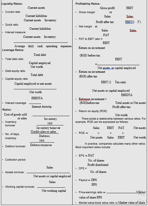
Review Questions

Explain the need for the financial analysis. How does the use of ratios help in financial analysis?
What do you mean by the liquidity of a firm? How can the liquidity of a firm be assessed?
Is it possible for a firm to have a high current ratio and still find difficulties in paying its current debt? Explain with illustration.
What are the leverage, or capital-structure, ratios? Explain the significance and limitations of the debt-equity ratio as a measure of the firm’s solvency?
Why are the activity ratios calculated? Do calculations of current asset turnover ratios indicate their quality? Explain.
How would you calculate the fixed assets turnover and the capital-employed turnover ratios? What do they imply?
Why is it necessary to calculate the profitability ratios in relation to sales? Illustrate your answer.
Explain the calculation and significance of the various measures of rate of return on investment.
Explain the ratios which you, as an analyst, will focus your attention to in the following cases:
- A bank is approached by a company for a loan of `50 lakh for working-capital purposes.
- A company requests a financial institution to grant a 10-year loan of `5 crore.
Which of the financial ratios of a company would you most likely refer to in each of the followingsituations? Give reasons.
- The company asks you to sell material on credit.
- You are thinking of investing `25,000 in the company’s debentures. (iii) You are thinking of investing `25,000 in the company’s shares.
What is the firm’s earning power? How are the net profit margin and the assets turnover related?
What is a DuPont analysis? Explain with the help of a chart.
‘A higher rate of return on capital employed implies that the firm is managed efficiently.’ Is thistrue in every situation? What or why not?
Ratios are generally calculated from historical data. Of what use are they in assessing the firm’sfuture financial condition?
Explain the significance and limitations of the ratio analysis.

(Visited 188 times, 1 visits today)

INTRODUCTION

USERS OF FINANCIAL ANALYSIS

NATURE OF RATIO ANALYSIS

Standards of Comparison

Types of Ratios

ILLUSTRATION 20.1: Assessing Financial Health of a Firm with Ratio Analysis

LIQUIDITY RATIOS

Current Ratio

Quick Ratio

Cash Ratio

Interval Measure

Net Working Capital Ratio

LEVERAGE RATIOS

Debt Ratio

Debt-Equity Ratio

Other Debt Ratios

Coverage Ratios

ACTIVITY RATIOS

Inventory Turnover

Debtors (Accounts Receivable) Turnover

Assets Turnover Ratios

PROFITABILITY RATIOS

Gross Profit Margin

Net Profit Margin

Net Margin Based on NOPAT

Return on Investment (ROI)

Return on Equity (ROE)

Earnings per Share (EPS)

Dividend per Share (DPS or DIV)

Dividend-Payout Ratio

Dividend Yield and Earnings Yield

Price–Earnings Ratio

Market Value-to-Book Value (MV/BV) Ratio

Tobin’s q

EVALUATION OF A FIRM’S EARNING POWER: DUPONT ANALYSIS

COMPARATIVE STATEMENTS ANALYSIS

TREND ANALYSIS

INTER-FIRM ANALYSIS

UTILITY AND LIMITATIONS OF RATIO ANALYSIS

Diagnostic Role of Ratios

CAUTIONS IN USING RATIO ANALYSIS

FINANCIAL RATIOS AS PREDICTORS OF FAILURE

Non-parametric Analysis

Multiple Discriminant Analysis

ILLUSTRATION 20.2: Z-Score

Review Questions

Written by MJ

Leave a Reply Cancel reply