Variance Analysis

BASIC VARIANCES

Knowledge brought forward from earlier studies

• A variance is the difference between an actual result and an expected result.
• Variance analysis is the process by which the total difference between standard and actual results is analysed.
• When actual results are better than expected results, we have a favourable variance (F). If actual results are worse than expected results, we have an adverse variance (A).
• The selling price variance measures the effect on expected profit of a selling price different from the standard selling price. It is calculated as the difference between what the sales revenue should have been for the actual quantity sold, and what it was.
• The sales volume variance measures the increase or decrease in expected profit as a result of the sales volume being higher or lower than budgeted. It is calculated as the difference between the budgeted sales volume and the actual sales volume multiplied by the standard profit per unit.
• The material total variance is the difference between what the output actually cost and what it should have cost, in terms of material(s). It can be divided into the following two sub-variances.
• The material price variance is the difference between what the material did cost and what it should have cost.
• The material usage variance is the difference between the standard cost of the material that should have been used and the standard cost of the material that was used.
• The labour total variance is the difference between what the output should have cost and what it did cost, in terms of labour. It can be divided into two sub-variances.
• The labour rate variance is the difference between what the labour did cost and what it should have cost.
• The labour efficiency variance is the difference between the standard cost of the hours that should have been worked and the standard cost of the hours that were worked.
• The variable production overhead total variance is the difference between what the output should have cost and what it did cost, in terms of variable production overhead. It can be divided into two sub-variances.
• The variable production overhead expenditure variance is the difference between the amount of variable production overhead that should have been incurred in the actual hours actively worked, and the actual amount of variable production overhead incurred.
• The variable production overhead efficiency variance is the difference between the standard cost of the hours that should have been worked for the number of units actually produced, and the standard cost of the actual number of hours worked.
• Fixed production overhead total variance is the difference between fixed production overhead incurred and fixed production overhead absorbed. In other words, it is the under– or over-absorbed fixed production overhead.
• Fixed production overhead expenditure variance is the difference between the budgeted fixed production overhead expenditure and actual fixed production overhead expenditure.
• Fixed production overhead volume variance is the difference between actual and budgeted production/volume multiplied by the standard absorption rate per unit.
• Fixed production overhead volume efficiency variance is the difference between the number of hours that actual production should have taken, and the number of hours actually taken (that is, worked) multiplied by the standard absorption rate per hour.
• Fixed production overhead volume capacity variance is the difference between budgeted hours of work and the actual hours worked, multiplied by the standard absorption rate per hour.

Exam Focus Point

You have to be very happy with basic variance calculations so it is essential to do more practice if you struggled with this question.

THE REASONS FOR VARIANCES

Knowledge brought forward from Formation 2 Management

Accounting

In an examination question you should review the information given and use your imagination and common sense to suggest possible reasons for variances.

Variance	Favourable	Adverse
Material price	Unforeseen discounts received Greater care taken in purchasing  Change in material standard	Price increase Careless purchasing Change in material standard
Material usage	Material used of higher quality than standard More effective use made of material Errors in allocating material to jobs	Defective material Excessive waste Theft Stricter quality control Errors in allocating material to jobs
Labour rate	Use of workers at a rate of pay lower than standard	Wage rate increase
Idle time	Possible if idle time has been built into the budget	Machine breakdown Non-availability of material Illness or injury to worker
Labour efficiency	Output produced more quickly than expected, because of work motivation, better quality of equipment or materials, better learning rate  Errors in allocating time to jobs	Lost time in excess of standard allowed Output lower than standard set because of lack of training, sub-standard material etc  Errors in allocating time to jobs
Overhead expenditure	Savings in costs incurred More economical use of services	Increase in cost of services Excessive use of services Change in type of services used
Overhead volume	Production or level of activity greater than budgeted.	Production or level of activity less than budgeted
Fixed overhead capacity	Production or level of activity greater than budgeted	Production or level of activity less than budgeted
Selling price	Unplanned price increase	Unplanned price reduction
Sales volume	Additional demand	Unexpected fall in demand Production difficulties

         

 

LABOUR VARIANCES AND THE LEARNING CURVE

Care must be taken when interpreting labour variances where the learning curve has been used in the budget process.

 

In Chapter 14 we looked at how the learning curve can be used for forecasting production time and labour costs in certain circumstances where the workforce as a whole improves in efficiency with experience.

Companies that use standard costing for much of their production output cannot apply standard times to output where a learning effect is taking place. This problem can be overcome in practice by:

• Establishing standard times for output, once the learning effect has worn off or become insignificant; and
• Introducing a ‘launch cost’ budget for the product for the duration of the learning period.

 

When learning is still taking place, it would be unreasonable to compare actual times with the standard times that ought eventually to be achieved so allowances must be made when interpreting labour efficiency variances. Standard costs should reflect the point that has been reached on the learning curve. When learning has become insignificant, standards set on the basis of this ‘steady state’ will be different to when learning was taking place. If the learning rate has been wrongly calculated, this must be allowed for in the variance calculations.

IDLE TIME AND WASTE

In the previous chapter we looked at the meaning of waste and idle time and how they can be allowed for in standards and budgets.  We now need to calculate their effect on variances.

Idle time variance

Idle time may be caused by machine breakdowns or not having work to give to employees, perhaps because of bottlenecks in production or a shortage of orders from customers. When it occurs, the labour force is still paid wages for time at work, but no actual work is done. Such time is unproductive and therefore inefficient. In variance analysis, idle time is an adverse efficiency variance.

The idle time variance is the number of hours that labour were idle valued at the standard rate per hour.

The idle time variance is shown as a separate part of the total labour efficiency variance. The remaining efficiency variance will then relate only to the productivity of the labour force during the hours spent actively working.

In Chapter 15 we discussed how budgets can be prepared which incorporate expected idle time. An adverse variance will only result from idle time in excess of what was expected.

Wastage and material variances

In the same way as idle time, a certain amount of expected wastage may be built into the material usage standard. A variance therefore needs to be calculated comparing the actual results with a standard that has been adjusted for expected wastage.

OPERATING STATEMENTS

Knowledge brought forward from earlier studies

• An operating statement is a regular report for management which compares actual costs and revenues with budgeted figures and shows variances.
• There are several ways in which an operating statement may be presented. Perhaps the most common format is one which reconciles budgeted profit to actual profit. Sales variances are reported first, and the total of the budgeted profit and the two sales variances results in a figure for ‘actual sales minus the standard cost of sales’. The cost variances are then reported, and an actual profit calculated.

Operating statements in a marginal cost environment  Knowledge brought forward from earlier studies

• There are two main differences between the variances calculated in an absorption costing system and the variances calculated in a marginal costing system. In a marginal costing system the only fixed overhead variance is an expenditure variance and the sales volume variance is valued at standard contribution margin, not standard profit margin.

ABC AND VARIANCE ANALYSIS

Within an ABC system, efficiency variances for longer-term variable overheads are the difference between the level of activity that should have been needed and the actual activity level, valued at the standard rate per activity.

All overheads within an ABC system are treated as variable costs, varying either with production levels in the short term or with some other activity. The traditional method of calculating fixed overhead variances is therefore not taken. The calculation of ABC overhead variances is either the same as the traditional approach for variable overheads (if the overhead varies with production level) or extremely similar (if it varies with some other activity).

Approach for longer-term variable overheads

Expenditure variances are the difference between what expenditure should have been for the actual level of activity and actual expenditure.

Efficiency variances are the difference between the level of activity that should have been needed and the actual activity level, valued at the standard rate per activity.

Usefulness of this analysis

Given the lack of relevant management information provided by traditionally-analysed fixed overhead variances, the results using ABC analysis are of more use. It is clear in the example above that one reason why the cost of the ordering activity was greater than it should have been given the level of production was because the cost per order was above budget. The main difference was because it took more orders than planned given the actual level of production, however. The analysis has highlighted the efficiency of the ordering process for investigation.

INVESTIGATING VARIANCES

Materiality, controllability, the type of standard being used, variance trend, interdependence and costs should be taken into account when deciding on the significance of a variance.

The decision whether or not to investigate

Before management decide whether or not to investigate the reasons for the occurrence of a particular variance, there are a number of factors which should be considered in assessing the significance of the variance.

Materiality

Because a standard cost is really only an average expected cost, small variations between actual and standard are bound to occur and are unlikely to be significant. Obtaining an ‘explanation’ of the reasons why they occurred is likely to be time consuming and irritating for the manager concerned. The explanation will often be ‘chance’, which is not, in any case, particularly helpful. For such variations further investigation is not worthwhile since such variances are not controllable.

Controllability

This must also influence the decision about whether to investigate. If there is a general worldwide increase in the price of a raw material there is nothing that can be done internally to control the effect of this. If a central decision is made to award all employees a 10% increase in salary, staff costs in division A will increase by this amount and the variance is not controllable by division A’s manager. Uncontrollable variances call for a change in the plan, not an investigation into the past.

The type of standard being used

The efficiency variance reported in any control period, whether for materials or labour, will depend on the efficiency level set. If, for example, an ideal standard is used, variances will always be adverse. A similar problem arises if average price levels are used as standards. If inflation exists, favourable price variances are likely to be reported at the beginning of a period, to be offset by adverse price variances later in the period.

 

Variance trend

Although small variations in a single period are unlikely to be significant, small variations that occur consistently may need more attention. Variance trend is probably more important that a single set of variances for one accounting period. The trend provides an indication of whether the variance is fluctuating within acceptable control limits or becoming out of control.

• If, say, an efficiency variance is RWF1,000,000 adverse in month 1, the obvious conclusion is that the process is out of control and that corrective action must be taken. This may be correct, but what if the same variance is RWF1,000,000 adverse every month? The trend indicates that the process is not out of control and may be the standard has been wrongly set.
• Suppose, though, that the same variance is consistently RWF1,000,000 adverse for each of the first six months of the year but that production has steadily fallen from 100 units in month 1 to 65 units by month 6. The variance trend in absolute terms is constant, but relative to the number of units produced, efficiency has got steadily worse.

 

Individual variances should therefore not be looked at in isolation; variances should be scrutinised for a number of successive periods if their full significance is to be appreciated.

Interdependence between variances

Individual variances should not be looked at in isolation. One variance might be inter-related with another, and much of it might have occurred only because the other variance occurred too. When two variances are interdependent (interrelated) one will usually be adverse and the other one favourable. 

 

 

Here are some examples.

Interrelated variances	Explanation
Materials price and usage	If cheaper materials are purchased for a job in order to obtain a favourable price variance, materials wastage might be higher and an adverse usage variance may occur. If the cheaper materials are more difficult to handle, there might be an adverse labour efficiency variance too. If more expensive materials are purchased, the price variance will be adverse but the usage variance might be favourable if the material is easier to use or of a higher quality.
Labour rate and efficiency	If employees are paid higher rates for experience and skill, using a highly skilled team might lead to an adverse rate variance and a favourable efficiency variance (experienced staff are less likely to waste material, for example). In contrast, a favourable rate variance might indicate a larger-than-expected proportion of inexperienced workers, which could result in an adverse labour efficiency variance, and perhaps poor materials handling and high rates of rejects too (and hence an adverse materials usage variance).
Selling price and sales volume	A reduction in the selling price might stimulate bigger sales demand, so that an adverse selling price variance might be counterbalanced by a favourable sales volume variance. Similarly, a price rise would give a favourable price variance, but possibly cause an adverse sales volume variance.

Costs of investigation

The costs of an investigation should be weighed against the benefits of correcting the cause of a variance.

Exam Focus Point

When asked to provide a commentary on variances you have calculated, make sure that you interpret your calculations rather than simply detail them.

Variance investigation models

The rule-of-thumb and statistical significance variance investigation models and/or statistical control charts can be used to determine whether a variance should be investigated.

Rule-of-thumb model

This involves deciding a limit and if the size of a variance is within the limit, it should be considered immaterial. Only if it exceeds the limit is it considered materially significant, and worthy of investigation.

In practice many managers believe that this approach to deciding which variances to investigate is perfectly adequate. However, it has a number of drawbacks.

• Should variances be investigated if they exceed 10% of standard? Or 5%? Or 15%?
• Should a different fixed percentage be applied to favourable and unfavourable variances?
• Suppose that the fixed percentage is, say, 10% and an important category of expenditure has in the past been very closely controlled so that adverse variances have never exceeded, say, 2% of standard. Now if adverse variances suddenly shoot up to, say, 8% or 9% of standard, there might well be serious excess expenditures incurred that ought to be controlled, but with the fixed percentage limit at 10%, the variances would not be ‘flagged’ for investigation.
• Unimportant categories of low-cost expenditures might be loosely controlled, with variances commonly exceeding 10% in both a favourable and adverse direction. These would be regularly – and unnecessarily – flagged for investigation.
• Where actual expenditures have normal and expected wide fluctuations from period to period, but the ‘standard’ is a fixed expenditure amount, variances will be flagged for investigation unnecessarily often.
• There is no attempt to consider the costs and potential benefits of investigating variances (except insofar as the pre-set percentage is of ‘material significance’).
• The past history of variances in previous periods is ignored. For example, if the pre-set percentage limit is set at 10% and an item of expenditure has regularly exceeded the standard by, say, 6% per month for a number of months in a row, in all probability there is a situation that ought to warrant control action. Using the pre-set percentage rule, however, the variance would never be flagged for investigation in spite of the cumulative adverse variances.

Some of the difficulties can be overcome by varying the pre-set percentage from account to account (for example 5% for direct labour efficiency, 2% for rent and rates, 10% for salesmen’s expenditure, 15% for postage costs, 5% for direct materials price, 3% for direct materials usage and so on). On the other hand, some difficulties, if they are significant, can only be overcome with a different cost-variance investigation model

Statistical significance model

Historical data are used to calculate both a standard as an expected average and the expected standard deviation around this average when the process is under control. An incontrol process (process being material usage, fixed overhead expenditure and so on) is one in which any resulting variance is simply due to random fluctuations around the expected outcome. An out-of-control process, on the other hand, is one in which corrective action can be taken to remedy any variance.

By assuming that variances that occur are normally distributed around this average, a variance will be investigated if it is more than a distance from the expected average than the estimated normal distribution suggests is likely if the process is in control. (Note that such a variance would be deemed significant.)

The statistical significance rule has two principal advantages over the rule of thumb approach.

• Important costs that normally vary by only a small amount from standard will be signalled for investigation if variances increase significantly.
• Costs that usually fluctuate by large amounts will not be signalled for investigation unless variances are extremely large.

 

The main disadvantage of the statistical significance rule is the problem of assessing standard deviations in expenditure.

 

Statistical control charts

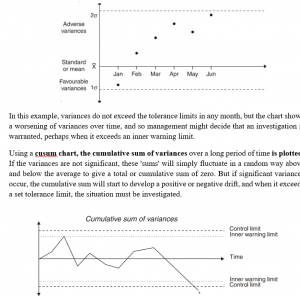
By marking variances and control limits on a control chart, investigation is signalled not only when a particular variance exceeds the control limit (since it would be non-random and worth investigating) but also when the trend of variances shows a progressively worsening movement in actual results (even though the variance in any single control period has not yet overstepped the control limit).

The x control chart is based on the principle of the statistical significance model. For each cost item, a chart is kept of monthly variances and tolerance limits are set at 1, 2 or 3 standard deviations.

 

 

 

The advantage of the multiple period approach over the single period approach is that trends are detectable earlier, and control action would be introduced sooner than might have been the case if only current-period variances were investigated.

Possible control action

Measurement errors and out of date standards, as well as efficient/inefficient operations and random fluctuations, can cause differences between standard and actual performance.

There are few basic reasons why variances occur and the control action which may be taken will depend on the reason why the variance occurred.

Measurement errors

In exam questions there is generally no question of the information that you are given being wrong. In practice on the factory floor, however, it may be extremely difficult to establish that 1,000 units of product A used 32,000 kg of raw material X. Scales may be misread, the pilfering or wastage of materials may go unrecorded, items may be wrongly classified (as material X3, say, when in reality material X8 was used), or employees may make ‘cosmetic’ adjustments to their records to make their own performance look better than it really was. An investigation may show that control action is required to improve the accuracy of the recording system so that measurement errors do not occur.

 

Out of date standards

Price standards are likely to become out of date quickly when frequent changes to the costs of material, power, labour and so on occur, or in periods of high inflation. In such circumstances an investigation of variances is likely to highlight a general change in market prices rather than efficiencies or inefficiencies in acquiring resources. Standards may also be out of date where operations are subject to technological development or if learning curve effects have not been taken into account. Investigation of this type of variance will provide information about the inaccuracy of the standard and highlight the need to frequently review and update standards.

Efficient or inefficient operations

Spoilage and better quality material/more highly skilled labour than standard are all likely to affect the efficiency of operations and hence cause variances. Investigation of variances in this category should highlight the cause of the inefficiency or efficiency and will lead to control action to eliminate the inefficiency being repeated or action to compound the benefits of the efficiency. For example, stricter supervision may be required to reduce wastage levels and the need for overtime working. The purchasing department could be encouraged to continue using suppliers of good quality materials.

Random or chance fluctuations

A standard is an average figure and so actual results are likely to deviate unpredictably within the predictable range. As long as the variance falls within this range, it will be classified as a random or chance fluctuation and control action will not be necessary.

MATERIALS MIX AND YIELD VARIANCES

The materials usage variance can be subdivided into a materials mix variance and a materials yield variance when more than one material is used in the product.

Manufacturing processes often require that a number of different materials are combined to make a unit of finished product. When a product requires two or more raw materials in its make-up, it is often possible to sub-analyse the materials usage variance into a materials mix and a materials yield variance.

Calculating the variances

The mix variance is calculated as the difference between the actual total quantity used in the standard mix and the actual quantities used in the actual mix, valued at standard costs.

The yield variance is calculated as the difference between the standard input for what was actually output, and the actual total quantity input (in the standard mix), valued at standard costs.

When to calculate the mix and yield variance

A mix variance and yield variance are only appropriate in the following situations.

• Where proportions of materials in a mix are changeable and controllable
• Where the usage variance of individual materials is of limited value because of the variability of the mix, and a combined yield variance for all the materials together is more helpful for control

 

It would be totally inappropriate to calculate a mix variance where the materials in the ‘mix’ are discrete items. A chair, for example, might consist of wood, covering material, stuffing and glue. These materials are separate components, and it would not be possible to think in terms of controlling the proportions of each material in the final product. The usage of each material must be controlled separately.

The issues involved in changing the mix

The materials mix variance indicates the cost of a change in the mix of materials and the yield variance indicates the productivity of the manufacturing process. A change in the mix can have wider implications. For example, rising raw material prices may cause pressure to change the mix of materials. Even if the yield is not affected by the change in the mix, the quality of the final product may change. This can have an adverse effect on sales if customers do not accept the change in quality. The production manager’s performance may be measured by mix and yield variances but these performance measures may fail to indicate problems with falling quality and the impact on other areas of the business. Quality targets may also be needed.

Alternative methods of controlling production processes

In a modern manufacturing environment with an emphasis on quality management, using mix and yield variances for control purposes may not be possible or may be inadequate. Other control methods could be more useful.

• Rates of wastage
• Average cost of input calculations
• Percentage of deliveries on time
• Customer satisfaction ratings
• Yield percentage calculations or output to input conversion rates

 

We will be considering performance measures in more detail in Study Unit 18.

CHAPTER ROUNDUP

• Care must be taken when interpreting labour variances where the learning curve has been used in the budget process.
• Within an ABC system, efficiency variances for longer-term variable overheads are the difference between the level of activity that should have been needed and the actual activity level, valued at the standard rate per activity.
• Materiality, controllability, the type of standard being used, variance trend, interdependence and costs should be taken into account when deciding on the significance of a variance.
• The rule-of-thumb and statistical significance variance investigation models and/or statistical control charts can be used to determine whether a variance should be investigated.
• Measurement errors and out of date standards, as well as efficient/inefficient operations and random fluctuations, can cause differences between standard and actual performance.
• The materials usage variance can be subdivided into a materials mix variance and a materials yield variance when more than one material is used in the product.