SPREADSHEETS MS – EXCEL

2.1 Definition of a spreadsheet

A spreadsheet is essentially a ledger sheet that lets you enter, edit and manipulate numeric data. There are two types of spreadsheets namely:

1. The manual spreadsheet.
2. The electronic spreadsheet.

A manual spreadsheet is the most commonly used type by book keepers as a ledger book with many sheets of papers divided into rows and columns on which various amounts of money are entered manually using a pen or pencil. You can visit your bursar’s office and request to see a ledger sheet.

An electronic spreadsheet on the other hand is prepared using a computer program that enables the user to enter values in rows and columns similar to the ones of the manual spreadsheet and to manipulate them mathematically using formulae.                                                        ‘

In this book, the word spreadsheet shall be used to refer to the electronic spreadsheet. ‘.

Advantages of Using Electronic Spreadsheets over Manual Spreadsheet

1. The electronic spreadsheet utilizes the powerful aspects of the computer like speed, accuracy and efficiency to enable the user quickly accomplish tasks.
2. The electronic spreadsheet offers a larger virtual sheet for data entry and manipulation. For example the largest paper ledger you can get is one that does not exceed 30 columns and 51 rows while with an electronic spreadsheet, the least ledger has at least 255 columns and 255 rows!
3. The electronic spreadsheet utilizes the large storage space on computer storage devices to save and retrieve documents.
4. The electronic spreadsheet enables the user to produce neat work because the traditional paper, pencil, rubber and calculator are put aside. All the work is edited on the screen and a final clean copy is printed. With a handwritten spreadsheet, neatness and legibility depends on the writer’s hand writing skills.
5. Electronic spreadsheets have better document formatting capabilities. 6. Electronic spreadsheets have inbuilt formulae called functions that enable the user to quickly manipulate mathematical data.
6. An electronic spreadsheet automatically adjusts the result of a formula if the values in worksheet are changed. This is called the automatic recalculation feature. For a manual sheet, changing one value means rubbing the result and writing the correct one again.

 

Examples of spreadsheets

1. VisiCalc: This was the first type of spreadsheet to be developed for personal computers.
2. Lotus 1-2-3: This is integrated software with spreadsheet module graphs and database. 3. Microsoft Excel
3. VP-Planner etc.

In this book, the spreadsheet that will be considered in details is Microsoft Excel.

Components of a spreadsheet

A spreadsheet has three components  ­

1. Worksheet.
2. Database.
3. Graphs.

Worksheet

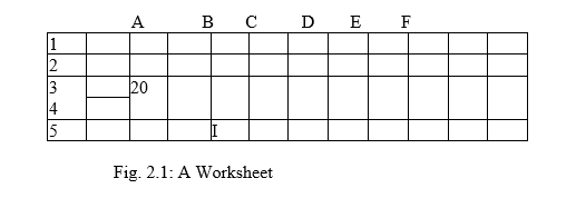
This is the component in which data values are entered. It is made up of rows and columns. The intersection between a row and a column is called a cell. A row is a horizontal arrangement of cells while a column is a vertical arrangement of cells. Each row is labeled with a number while each column is labeled with a letter as shown in the Figure 2.1. Each cell is referenced using the column label followed by the row label e.g. cell B3 has the value 20. A group of many worksheets make up a workbook.

Database

Data values can be entered in the cells of the spreadsheet and managed by special Excel features found on the Data menu. These features were incorporated in Excel but they actually belong to database management software. One of such feature is filtering records, using forms, calculating subtotals, data validation pivot tables and pivot chart reports.

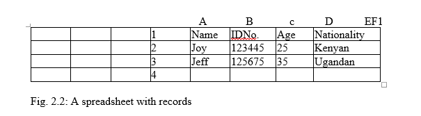
If the data values for the same entity (related values) are entered on the same row, they form a record. Hence a worksheet can be manipulated to some extent as a database that has data records entered in it. Figure 2.2 shows a worksheet having two records, Joy and Jeff.

NB: A spreadsheet file is structured in such a way that it can be visualised as a table of records. That is why such a ‘file can be imported into a database program as will be discusses later in databases.

 

Graphs

A graph is a pictorial representation of the base data on a worksheet. Most spreadsheets refer to graphs as charts. A chart enables the user to present complex data elements from a worksheet in a simple easy to understand format. Examples of charts are pie charts, line charts and bar charts. As shall be discussed later, it is easy to generate charts when working with a spreadsheet program. Figure 2.3 shows an example of a pie chart.

 

2.3 Application areas of a spreadsheet 

Statistical analysis

Spreadsheets provide a set of data analysis tools that can be used to save steps when developing complex statistical or engineering analyses. The user is usually expected to provide the appropriate data and parameters for each analysis. The statistical tool then uses appropriate automated statistical or engineering functions and then displays results in an output table. Some of the tools generate charts in addition to the output tables.

Because most of these tools are complex, the user needs to have the statistical background knowledge before attempting to use the tools. Examples of some simple statistical functions include the following:

1. Average: This is used to calculate the mean of a set of values.
2. Median: This is used to return the value in the middle of a set of values.

For example a set of values may be composed of:

10   20    30   40    50     60.

The average of the set is 35 and its median is also 35. The median is found by taking the average of the two numbers at the centre of the set, in this case 30 and 40.

Accounting

Many accountants find the spreadsheet a useful tool to use in recording daily transactions and keeping of financial records. Spreadsheets provide a user friendly environment for financial management and they come with inbuilt functions that make accounting tasks easier. For example, the spreadsheet can be used by accountants to do the following:

1. To track the value of assets over time (depreciation and appreciation)
2. To calculate profits
3. To prepare budgets

Other formula like sum, average, product etc. enables the accountant to carry out his daily work without any problem.

Data management

A spreadsheet enables neat arrangement of data into tabular structure. Related data can be typed on the same worksheet. However, when data is on different worksheets, the worksheets can be linked to enhance accessibility.

Data management functions include sorting, filtering (displaying only the required items) and using forms to enter and view records.

Spreadsheets enable the user to create, edit, save, retrieve and print worksheet data and records.

Forecasting (“What if” analysis)

The automatic recalculation feature enables the use of “What if’ analysis technique. This involves changing the value of one of the arguments in a formula to see the difference the change would make on the result of the calculation. For example, a formula to calculate a company’s profit, margin may be as follows:

Profit =, (Total units sold x sale price) – (Total units bought x cost price)     – Operating ‘expenses.

A sales manager in the company c n ask the following question: What if sales increase by 20%, how much profit wills the company make? The manager substitutes the total units sold value with one that is 20% higher and the spreadsheet automatically displays the new profit. A traditional analysis method would require a different work sheet to be prepared. Therefore, this method can be used for financial forecasting, budgeting, stock portfolio analysis, cost analysis, cash flow etc.

Creating a worksheet/workbook using Microsoft Excel

To start Microsoft Excel, click Start button, point to Programs and then select Microsoft Excel from the programs menu This procedure may vary slightly depending on the version of Excel you are using or the computer’s hardware and software configuration.

The Windows environment allows a person to place shortcuts to a program’s executable (.exe) file in various places like the desktop. If the Excel shortcut is on the desktop, simply double click it to start the application.

The Microsoft Excel application window opens as shown in the Figure 2.5. Make sure that you can be able to identify all the labeled parts of the Microsoft Excel application window.

The Microsoft Excel application window

The Microsoft Excel application window is made up of the following components:

Title bar: It has the title of the application and control buttons for minimising, maximising and closing the application

The menu bar: It displays a list of menu options e.g. File, Edit, View etc. Clicking one of them displays a menu that has commands which can be selected in order to manipulate data in the spreadsheet.     ‘

Tool bars: The most common of these are the standard and formatting toolbars. The most important thing is to be able to identify each toolbar by its icons. The standard toolbar has shortcuts to some of the most commonly used menu commands like print, copy, paste and save. The formatting toolbar has shortcuts to the commonly used commands found on the format menu option

Formula bar: This is one of the most important components of the Microsoft Excel application window. It enables the user to enter or edit a formula or data in a cell. You can identify the formula bar because it has an equal sign (or fx). The name box to the left of the formula bar displays the position of the cell in which data or a formula is being entered which is also called the current cell. If the formula bar is not available, click on View menu then select Formula bars. A check mark appears on the left of the selected item to show that it is now displayed on the screen.

Cell pointer: It marks the position of the current cell or the insertion point. It is special cursors that is rectangular in shape and makes the current cell appear as if it has darker boundaries.

The Worksheet: Consists of cells, rows and columns. Data is entered here for manipulation.

Status bar: It shows the processing state of the application. For example, on its left is the word Ready which shows that the spreadsheet is ready to receive user commands.        ‘

Worksheet labels: These are usually of the format Sheet 1, Sheet 2 etc. A workbook may have several sheets. It is also possible to rename the sheets by right clicking on the labels then choosing rename command from the shortcut menu that appears. The active sheet (one being used) has its label appearing lighter in colour than the rest. To move to a particular sheet in the workbook, simply click its sheet label.

Vertical and horizontal scroll bars: Clicking the arrows at their ends moves the worksheet vertically and horizontally on the screen respectively.

 

Worksheet layout

The worksheet has the following components: Cells: An intersection between a row and a column.

Rows: Horizontal arrangement of cells. Columns: Vertical arrangement of cells.

Range: Is a group of rectangular cells that can be selected and manipulated as a block.

 

Navigating the Microsoft Excel screen

1. Click cell D5. Notice that the cell pointer immediately moves to the cell and the name box reads D 5. Typing on the keyboard now inserts entries in cell D5 as long as the pointer is still there.
2. Click letter A that heads the first column. Notice that the whole column is highlighted.
3. Double click cell EIO. Notice that the text cursor forms in the cell and you can now type characters inside the cell. Also the status bar will now read enter which means that Microsoft Excel expects you to enter a value in the cell.
4. Click the down arrow on the vertical scroll bar. The worksheet moves upwards on the screen. The opposite happens when you click the up arrow on the vertical scroll bar.
5. Click the right button on the horizontal scroll bar. The worksheet moves to the left. The opposite happens when you click the left button on the horizontal scroll bar.
6. Press the right arrow key on the keyboard. Notice that the cell pointer moves one column to the right on the same row. This can also be done by pressing the Tab key once.
7. Press the left arrow key on the keyboard. Notice that the cell moves one column to the left on the same row. Pressing gives the same results.
8. Press the up arrow key on the keyboard. Notice that the cell pointer moves one row up on the same column.
9. Press the down arrow key on the keyboard. Notice that the cell pointer moves one row down on the same column.
10. Press the end key. The status bar will display the message “END”. If you press the right arrow key, the cell pointer will move right to the last cell on the row. If the left up or down keys were to be pressed instead, the cell pointer would move to the last cell to the left, top or bottom respectively.
11. Pressing Ctr1+Home moves the cell pointer to the first cell of the worksheet i.e. cell AI.

 

Creating a worksheet

At its simplest level, creating a worksheet consists of starting the spreadsheet program and entering data in the cells of the current worksheet. , However, a person can decide to create a worksheet either using the general format or from a specially preformatted spreadsheet document called a template.

 

Using the general format

When a spreadsheet program is running it will present the user with a new blank screen of rows and columns. The user can enter data in this worksheet and save it as a newly created worksheet. If this is not available then click File menu option and select the new command. The dialog box shown in Figure 2.8 will be displayed on the screen. On the General tab, double click the workbook icon. Enter data in the new worksheet created.

 

Using a template

Click File menu option then new command. On the spreadsheets solutions tab, double click the template that you wish to create. Figure 2.9 below shows some examples of templates that may be present for selection.

 

NB: If the template was saved previously on the hard disk, it will open as a new worksheet with all the preformatted features present allowing the user to enter some data. However, some templates may require the original program installation disk in order to be able to use them because they may not have been copied to the hard disk during program installation.

 

Editing a cell entry

Editing a cell means changing the contents of the cell. Before the contents in a cell can be. Changed, the cell must be selected by making it the current cell.

To edit a cell entry proceeds as follows:

1. Move the cell pointer to the cell you wish to edit.
2. Double click the formula bar for the text cursor to appear in the bar. The status bar message changes to edit
3. Use the keyboard to delete and add contents to the formula bar then press enter key to apply. Click the save button on the standard toolbar to save the edited changes.

 

Selecting a range

As you have experienced with the previous two examples, working with one item at a time is tedious and time consuming. Using a range saves time when working with a large .amount of data.

 

A range is a rectangular arrangement of cells specified by the address of its top left and bottom right cells, ‘separated by a colon (:) ego Range AI:CIO is as shown in Figure 2.10.

Selecting multiple ranges

When using a mouse, you can select more than one range without removing the highlight from the previous. To do this:

Hold down the Shift key or the Ctrl key while you click on the row header of the second range you want to highlight. What happens? Do you notice the difference when holding down the shift and the ctrl keys?

1. Shift key will cause all columns/rows between the selected and the newly clicked cell to be highlighted.
2. Ctrl selects individually clicked cells or range.

 

Hiding rows/columns

You can hide some rows or columns in order to see some details, which do not fit, on the screen. To do this:

1. Highlight the columns/rows you want to hide
2. Click format menu, point on row or column and click hide command.

 

Saving a worksheet

To save a worksheet, one has to save the workbook in which it belongs with a unique name on a storage device like a hard disk. The procedure below can be used to save a workbook:

1. Click File menu option then select Save as’ command. Alternatively, click the save command on the standard toolbar. The save as dialog appears
2. Select the location in which your workbook will be saved in the Save in box then type a unique name for the workbook in the File name box. Make sure that the option Microsoft Excel Workbook is selected under the save as type box.
3. Click the Save button to save.

 

Retrieving a saved workbook

This means opening a workbook that was previously saved.

1. Click File menu option then the Open command. Notice that the Open command has three dots (called ellipsis) indicating that a dialog box will open, as the user is required to provide additional information. Alternatively just click the Open command on the standard toolbar. The open dialog box appears on the screen.
2. Click the Look in drop down list arrow and select the drive or folder where the workbook was saved. For example, if you saved in a diskette, insert it in the floppy drive then select 3 1/2-floppy (A:). A list of folders and files in the drive will appear in the list box.
3. Double click the icon of the workbook you want and the worksheet will be displayed in the Microsoft Excel window. Notice that the cell pointer is in the same cell it was in when the worksheet was last Saved.

Closing a worksheet

Click File then Close command. This closes the worksheet but does not

Close the Excel spreadsheet program. Alternatively, click the; close button of the worksheet window

Exiting from the spreadsheet                  

Click File then Exit command. This closes not only the worksheet but also the spreadsheet program as well. Alternatively click the close button of the main application window.

Cell data types

There are four basic types of data used with spreadsheets:

1. Labels
2. Values,
3. Formulae
4. Functions.

 

Labels

Any text or alphanumeric characters entered in a cell are viewed as labels by the spreadsheet program. Labels are used as row or column headings usually to describe the contents of the row or column. For example, if a column will have names of people, the column header can be NAMES. Sometimes, numbers can be formatted so that they can be used as labels. To achieve this add an apostrophe just before the most significant digit in the number. For example, the number 1990 will be treated as numeric. if typed in a cell but’ 1990 will be treated as a label.

Labels are aligned to the left of the cell and cannot be manipulated mathematically.

 

Values

These are numbers that can be manipulated mathematically. They may include currency, date, numbers (0-9), special symbols or text that can be manipulated mathematically by the spreadsheet.

 

Formulae

These are user designed mathematical expressions that create a relationship between cells and return a value in a chosen cell. In Microsoft Excel, a formula must start with an equal sign. For example, the formula

=B3+D4 adds the contents ofB3 and D4 and returns the sum value in the current cell.

Excel formulae use cell addresses and the arithmetical operators like plus (+) for addition, minus (-) for subtraction, asterisk (*) for multiplication and forward slash (I) for division.

Using cell addresses, also called referencing, enables Microsoft Excel to keep calculations accurate and automatically recalculates results of a formula in case the value in a referenced cell is changed. This is called automatic recalculation.

 

Functions

These are inbuilt predefined formulae that the user can quickly use instead of having to create a new one each time a calculation has to be carried out Microsoft Excel has many of these formulae that cover the most common types of calculations performed by spreadsheets. To add the contents of cell B3 and D4 the sum function can be used as shown below:

= Sum (B3:D4)

 

Cell referencing

A cell reference identifies a cell or a range of cells on the worksheet and shows Microsoft Excel where to look for the values or data needed to use in a formula. With references, you can use data contained in different cells of a worksheet in one formula or use the value from one cell in several different formulae.

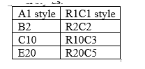
By default, Microsoft Excel uses the A 1 cell referencing style. This means that a cell is identified by its column label followed by the row number. However, the Rl Cl referencing style can be used. In this case, the cell is referencing by its row number followed by its column number. The table below gives a few examples of equivalent referencing using both styles.

The RlCl style is useful when automating commonly repeated tasks using special recording programs called Macros.

Relative referencing

When performing tasks that require cell referencing, you can use formulae whose cell references keep on changing automatically depending on their position in the worksheet. This is called relative cell referencing. A good example would be if you type the formula =Al+Bl in cell Cl. If the same formula is copied to cell C2 the formula automatically changes to =A2+B2.

 

Absolute referencing

These are cell references that always refer to cells in a specific location, of the worksheet even if they are copied from one cell to another. To make a formula absolute, add a dollar sign before the letter and/or number, such as $B$lO. In this case, both the column and row references are absolute. .

 

Referencing using labels and names

Labels of columns and rows on a worksheet can be used to refer to the cells that fall within those columns and rows. It is possible to create a name that describes the cell or range then use it instead of having to specify a range with actual cell references. Such a descriptive name in a formula can make it readable and easier to understand its purpose. For example, the formula =SUM(SecondQuarterProfits) might be easier to identify than =SUM(AlO:C20). In this example, the name SecondQuarterProfits represents the rangeAlO:C20 on the worksheet. Names can also be used to represent formulae or values that do not change (constants). For example, you can use the name .Tariffs to represent the import tax amount (such as 7.0 percent) applied to imports.

 

To create a named range

To create a named range proceeds as follows:

1. Select the range to be named:
2. Click inside the name box to move the text cursor inside. Delete the Cell reference that is there and type a name for the range.
3. Press Enter key to apply. Figure 2.13 shows a worksheet range called sales that has values used in a formula to give the sum in cell C 11.

 

2.7 Basic functions and formulae

Formulae perform mathematical operations ranging from very simple arithmetic problems t9 complex scientific, financial and mathematical analysis.

 

Statistical functions.

1. Average: It returns the average (mathematical mean) of a set of values which can be numbers, arrays or references that contain numbers. If the value 20 is in cell DIO and 30 in ElO then:

=Average(D lO:E 1 0) returns 25 as the average of the two values.

2. Count: Counts the number of cells that contain values within a range e.g.

= count (AIO: EIO) many return a value 5 if all the cells have values.

3. Max: It returns the largest value in a set of values. It ignores text and logical values e.g. == Max (AlO:EIO) will return the maximum value in the range.
4. Min: It returns the smallest value in a set of values. It ignores text and logical values e.g. = Min (AIO:EIO) will return the minimum values in the range.
5. Mode: It returns the most frequently occurring value in a set of values. e.g. = Mode (AIO:ElO)
6. Rank: Returns the rank of a number in a list by comparing its size relative to the others. For example if A 1 to AS contains numbers 7, 3.8,3.8, 1 and 2 then RANK (A2, Al :A5,1) returns 3 while RANK (AI, AI:A5,I) returns
7. The general format is RANK (number to be ranked, range, order).

 

Logical functions

1. If: It returns a specified value if a condition is evaluated and found to be true and another value if it is false. If (marks > 50, “pass”, “fail”) will display a pass if values are more than 50 else it will display fail.
2. Countif: Counts the number of cells within a specified range that meet the given condition or criteria. e.g. suppose A 1 0 : E 1 0 contains eggs, beans, beans, eggs, eggs, countif(AIO:EIO, “Eggs”) will return 3.
3. Sumif: It adds values in the cells specified by a given condition or criteria. e.g. For example if AIO to ElO contains values 10,50,60, 30, 70, to sum all values greater than 50 = Sumif(AIO:EIO, “>50”). This returns 130.

 

Mathematical functions

1. Sum: adds values in a range of cells as specified and returns the result in the specified cell. e.g Sum (AIO:EIO) adds values in the range
2. Product: multiplies values in a range of cells and returns the result in the specified cell. For example if A 10 has 30 and BIO has
3. Product (AlO:BIO) will return 90.

 

Arithmetic formulae – using operators

       Operator Function

 

+ (plus)                                          adds values as specified

– (minus) .                                      subtracts values as specified

* (multiplication)                           multiplies values

/ (division)                                      divides values.

( ) parenthesis                                      encloses arguments to be calculated first.

 

For a formula =(Al +C3)/E20, if the value in E20 is not zero, the result is displayed in the current cell.

 

Order of execution

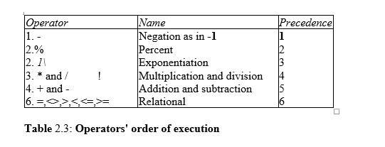
If several. Operators are used in a single formula; Microsoft Excel performs the operations in the order shown in Table 2.3. Formulas with operators that have same precedence i.e. if a formula contains both a multiplication and division operator are evaluated from left to right. Enclosing part of the formula to be calculated in parentheses or brackets makes that part to be calculated first.

2.8 Editing a worksheet

 Coping and moving data

Spreadsheet software automates many processes that could have been tedious if done manually. For example with Microsoft Excel, you can do calculations using formulae fairly easily as you give the data and correct instructions to the program. Copying and moving of, data can also be done quickly and efficiently.

When data is cut or copied from the worksheet, it is temporarily held in a storage location called the clipboard.

 

Copying data

To copy a cell or a range of cells:

1. Highlight the cells or range you want copied
2. Click the Edit menu then select Copy command.
3. Select the cell in which you want to place a copy of the information 4. From the Edit again, click Paste command. The Paste command puts a copy from the clipboard on the specified location

 

Moving data

Unlike the Copy command where a duplicate copy is created, the Move command transfers the contents of the original cell (s) to a new location.

 

To move a range of cells:

1. Highlight the range you want to move.
2. From the Edit menu, select Cut.
3. Specify the location you want to move the contents to.
4. From the Edit menu again, click Paste.

 

2.9 Worksheet formatting

Worksheet formatting refers to enhancing the appearance of the worksheet to make it more attractive and appealing to the reader. Appropriate formatting should be used to lay emphasis, catch attention and bring otherwise II hidden detail to the fore of the document.

The golden rule of formatting is to use simple clear formats. It essentially consists of changing text colour and typeface (font), size, style and alignment. In Microsoft Excel, format the cells whether empty or not and their contents will acquire the set format automatically.

To format a single cell, make it the current cell then format menu option and select the cells command In the format cells dialog box, make the formatting specifications that you wish then click the ok button to apply. If it is a range of cells, they must be highlighted first before formatting them as a block of cells.

Formatting text

1. Highlight the cells that have the text to be formatted.
2. Click Format menu then cells command. The dialog box appears
3. Select the font tab as shown in the figure by clicking it.
4. Select the font type e.g. Times New Roman. Other font formatting features like style, size, underline and colour are available and can be selected.
5. Click button to apply.

 

NB: Alternatively, use the formatting toolbar to accomplish all your text formatting needs. Notice that the options in the font dialog box are commands on the formatting toolbar.

 

Formatting numbers

1. Highlight the cells that have the numbers to be formatted.
2. Click Format menu then cells command. The dialog box in Figure 2.15 appears.
3. Select the Number tab as shown in the figure below.
4. You can now choose number formats as explained below:

Number            Meaning

General            general format cells have no specific number format.

Number           Used for general display of numbers e.g. 2345.23.

Currency         For displaying general monetary values e.g. $100, Ksh.10.

Accounting     Lines up the currency symbols and decimal poin s. Displays date in chosen format.

Date                Displays time in chosen format.

Percentage       Multiplies the value in a cell with 100 and display ‘ it as %.

Text                 Formats cells to be treated as text even when numbers are entered.

Custom          For a number format not predefined in Microsoft Excel, select custom then define the pattern.

 

Worksheet borders

You may need to put a printable border around your worksheet or in a range of cells to make it more attractive and appealing. To put a border:

1. Highlight the range you wish to insert borders. From the format menu, click cells command.
2. Click the borders tab and specify the border options for left, right, top and bottom. .
3. From the style options, select the type of line thickness and style. Also select the preset options.
4. Click the ok button. The selected range will have a border around it.

 

Formatting rows and columns

Sometimes, the information entered in the spreadsheet may not fit neatly in the cell set with the default height and width. It therefore becomes necessary to adjust the height of a row or the width of a column. The standard width of a column in Microsoft Excel is 8.43 characters but can be adjusted to any value between 0 and 255.

 

Changing column width

1. Move the mouse pointer to the right hand side line that separates the column headers i.e. for instance the line between A and B.
2. Notice that the mouse pointer changes from a cross to a double arrow
3. Click the mouse button and hold it down so that you can now resize the width of the column by dragging to the size you wish. After Dragging to the required point release the mouse button and the Column will have a new size.

 

NB: Alternatively, move the cell pointer to one of the cells of the column then click Format, point to Column then click Width command from the sidekick menu. Type a width in the dialog box that resembles Figure 2.17 then click Ok.button to apply.

NB: To change the widths of several columns at the same time, highlight them first before following this method.

 

Changing row height

1. Point to the line that separates two row numbers e.g. the line between 1 and 2. The mouse pointer becomes a double arrow.
2. Drag the line until the height of the row is as required then stop and release the mouse button.

NB: Alternatively, click Format point to Row then click Height from the sidekick menu that appears. Type the height that you wish in the dialog box that appears and then click OK button to apply.

 

Inserting rows and columns

I, Click cell A5 to make it the current or active cell.

2.clik insert then columns to insert a ‘row above cell A5 and shift all the other rows downward.

OR

 Click insert then Columns to insert a column to the left of column A and shift all the others to the right.

NB: Alternatively, click  insert  then cells to display the dialog box select the entire row or entire column options to insert a row or column respectively.

 

Global worksheet formatting

The word global in this case refers to the entire worksheet. In order to format the whole worksheet globally, it must be selected as a whole.

Two methods can be used to select a worksheet globally:

1. Click the top left comer of the worksheet that has a blank column header i.e. immediately on the left of A and just above I,

OR

2. Press Ctrl+A on the keyboard.

 

Notice that the whole worksheet becomes highlighted. It can now be formatted as one big block using format cells command.

 

Using autoformat

It allows the user to apply one of sixteen sets of formatting to & selected range on the worksheet. This quickly creates tables that are easy to read and are attractive to the eye..

1. Select a range e.g. B 1 :G7 to make it active.
2. Click format then select the auto format command on the menu that Appears. Select a format from the autoformat dialog box shown in Figure 2.19.
3. Click the ok button to apply the format to the selected range.

 

2.9 Data management

At times, it becomes necessary to use advanced data management tools to manage large ,data stored on a ‘worksheet. For example, if the worksheet has many records, it may become necessary to arrange them in a particular order using a method called sorting for easier access to data items. Other methods of data management include use of filters, total/subtotal function and forms.

 

Sorting

To carryout sorting proceed as follows:

1. Highlight the range that you wish to sort by clicking its column header letter.
2. Click Data then Sort . Notice that the Sort by field is already reading the field that you selected. This field is called the criteria field.
3. Select the field to be used as the key for sorting and the sort order as either descending or ascending then click OK button to apply.

 

Filtering data

Filtering is a quick and efficient method of finding and working with a subset of data in a list. A filtered list will only display the rows that meet the condition or criteria you specify. Microsoft Excel has two commands for filtering lists.

1. The auto filter: It uses simple criteria and includes filter by selection.
2. Advanced filter: It uses more complex criteria.

In this Pupil’s Book we will look at the autofilter.

 

Autofilter

Filters can be applied to only one list on a worksheet at a time.

1. Click a cell in the list that is to be filtered; usually the list is in a column.
2. On the Data menu, point to Filter, and then
3. To display only the rows that contain a specific value, click the arrow in the column that contains the data you want to display as shown in Figure 2.21.
4. Click the value that is to be displayed by the filter from the drop down list. e.g in the example below, the selected value is 34.

NB: Sometimes while looking through a list of values on a large worksheet, you may come to a value of interest and want to see all other occurrences of the value in the spreadsheet. Simply click the cell that has the value then click auto filter on the standard toolbar. Microsoft Excel turns on AutoFilter and then filters- the list to show only the rows you want.

 

Subtotals function

Consider the following scenario: A company that has many salespersons

will need to know how much each of them should be paid at the end of a period by looking at individual sales volumes. Also, the grand total for all the payments has to be calculated. Therefore, if the salespersons are held in a list, there would be need to calculate the amount due to each of them. This can be called a subtotal in the list. All the subtotals can then be added together to make the grand total. Consider the following list:

Name                    Amount Owed

Stephen           `           6000

Joy                               3000

Stephen                      2000

Virginia                      5000

Joy                              800

Stephen                       200

Virginia                      5000

 

Microsoft Excel can automatically summarise the data by calculating subtotal and grand total values of the list. To use automatic subtotals, the list must have labelled columns and must be sorted on the columns for which you want subtotals. In this example, the list is first sorted by name

1. Click a cell in the list that will have subtotals e.g. cell A3.
2. On the Data menu click Subtotals 3. Notice that all the data range is now selected.
3. In each change in box, select Name from the drop down list because we want a subtotal for each of the names.
4. In the Use function box select the sum function then select the list for which subtotals will be inserted in the add subtotals box by checking the appropriate label. In this case it is the amount owed field.
5. Click ok button to apply and the list will now have sub totals inserted

Totals function

Use theAutoCalculate feature in Microsoft Excel to automatically show the total of a selected range. When cells are selected, Microsoft Excel displays the sum of the range on the status bar. Right clicking this function displays other functions like Min, Max and Average that can also be used. To find the total of a range, highlight it then click the autosum icon ∑ on the standard toolbar.

 

Forms

A form is a specially prepared template that the users can use to enter data in a worksheet. It is specifically formatted to enable users to enter data in a format that is more convenient to them. If data is collected on paper before entering in the computer, then a form can be created to have the layout of the data on the paper to quicken data entry procedures. To display a form: Click ‘Data, then form.

 

2.10 Charts/graphs

Charts/graphs are graphics or pictures that represent values and their relationships. A chart helps the reader to quickly see trends in data and to be able to compare and contrast aspects of data that would otherwise have remained obscure. Microsoft Excel has both two-dimensional and 3-dimensional charts that can be used instead of the raw data in the table that has to- be studied for a long time to understand it.

The various types of charts available include column, bar, line. Pie, bubble and area charts among others. Consider carefully the type of chart that would best represent the base data in the worksheet before creating one. For example, if the aim is to depict the performance index of a student from Form I-to 3, a line chart would be most appropriate because it clearly shows the trend in performance.

Types of charts

1. Line chart – represents data as lines with markers at each data value in the x-y plane.
2. Column chart- represents data as a cluster of columns comparing values across categories. .
3. Bar chart – data values arranged horizontally as clustered bars. Compares values across categories.
4. Pie chart – it displays the contribution of each value to a grand total.
5. Scatter chart – compares pairs of values on the same axis.

To view types of charts, right click the chart object then select the chart type command.

 

Creating a chart

A chart must be based on values that are already entered in the worksheet.

 

To create a chart:

1. Select the range of values for which you want to create a chart.
2. Click the Chart wizard button on the standard toolbar and the chart wizard dialog box will open as shown in Figure 2.25
3. Click the type of chart you wish to .create. If the office assistant appears, close it. The chart sub-type preview will show several styles of the selected chart type.
4. Click the Next button to move to the dialog in Figure 2.26.
5. Click the Series tab then the collapse dialog button on the labels text box.

This will shrink the dialog box so that only the category labels text box is shown. Highlight the data labels from the worksheet.

6. Click the Expand dialog button to bring the full dialog box into view then click the: Next button. In step 3 of the wizard, use the appropriate tabs to type the title of the chart, show a legend, select whether to display gridlines or not etc. After all these click the Next button.’
7. At step 4 determine whether the chart will be inserted in the current worksheet or a new worksheet then click Finish button (Figure 2.27).

 

Moving and resizing a chart

Once the chart is created, its size and location can be changed in the worksheet. The chart element is enclosed inside a boundary called the chart area and hence both can be resized independently. Simply click the object you wish to resize and use the object handles just like in objects to drag to size. To move the chart, click inside the chart area then drag to the desired position.

 

Data ranges

A data range is a rectangular block of cells that provides the base data that is used to create the chart. In charting, a data range is referenced as an absolute range e.g. .

=Sheetl !$B$2:$C$8 which means that the base data is found on Worksheet 1 and absolute range B2:C8.

To see the data range of a chart, right click it then select the Source data command. .

 

Labels

Each representation of data on a chart can either be labelled by a value

or text label. For example, in a bar chart that compares the height of pupils, each bar can be given a value label to make it more readable.

 

To label:

1. Right click the chart then select the Chart options command from the shortcut menu.

2. Click the lables tab and choose whether you want value or text labels then click OK button to apply. .

 

Headings and titles

Each chart must have a heading showing clearly what it represents. To I make the chart understandable, include axis titles.

To include axis titles proceed as follows:

1. Right click the chart then select the. Chart options command.
2. Click the Titles tab then type the chart title (heading). And axis titles respectively.
3. Click OK button to apply.

 

Legends

The legend is like a key that explains what each colour or pattern of the data representation in the chart means. For example, Microsoft Excel may give red colour to one data value and green to the other. Without a legend it would be difficult to know how to differentiate the two sets of values.

To create a legend:

1. Right click the chart then select the Chart options command.
2. Click the legends tab and specify that it be displayed in the chart area.
3. Click OK button to apply.

 

2.11 Printing worksheets

A worksheet will finally be printed for sharing with others or for filing purposes. If it contains objects like charts, it may not fit on a standard printing page using the default printing options and settings. Therefore, Microsoft Excel allows the user to preview and set up the pages of a’ worksheet in order to fit them on the hard copy page.

 

Page setup

1. Click .File menu option then Page setup command to display the page setup dialog box. . .
2. On the Page tab, select the orientation of the page. Study the meanings of each buttons and options in Figures 2.28.
3. After making the necessary selections, click OK to apply.

 

Print preview

It displays the worksheet from the point of view of the printer i.e. exactly the way it will look when printed. Before using this command, make I sure the chart is deselected.

1. Click the Print preview button on the standard toolbar.
2. The worksheet will be displayed in the print preview window with the status bar reading preview.
3. Click Setup to start the page setup dialog box. To close the preview, click the Close. Button.

Print options

 To print click File then Print command. The print dialog, box appears as shown in Figure 2.29 .

1. Select printer – the name box in this dialog box enables a person to select the printer that will be used to print the document. All the printers that are installed on the computer will be available here.
2. The print what options are:

Selection – this prints the selected worksheet area.

Workbook – prints all the worksheets in the workbook.

Selected chart – prints the selected chart only.

 

Page orientation

As explained earlier, page orientation refers to the layout of the text on the page. A worksheet can also be printed on either landscape or portrait depending on the number of columns across the worksheet.

 

Pages and copies                                                                         .

The number of copies box specifies how many copies of a particular worksheet or workbook should be printed.

Sometimes only some specified pages in a workbook are specified for printing e.g. if a workbook has 100 pages and you wish to print only pages 50 to 60 select the page(s) range button then type 50 and 60 in the from, to boxes respectively before clicking the OK button.

 

Printing

After selecting all the options, click the OK button to print.

 

Some common printing problems

1. A message appears on the screen saying that the printer specified could not be found in the directory.

 

Possible problems and solutions

1. The printer could be off. Switch it on and it will start printing.
2. The data cable to the printer could be loose. Make sure it is firm at the ports.
3. The wrong printer could have been selected. Select the right one in the print dialog box and send the print job again.
4. A message appears on the screen reading that there is paper jam.

The printer is clogged with a paper jam. Alert the lab, technician or the Teacher to clear the paper jam.