
ANALYSING FIXED AND VARIABLE COSTS
Two important quantitative methods the management accountant can use to analyse fixed and variable cost elements from total cost data are the high-low and regression methods.
The high-low method
You will have encountered the high-low method in your earlier studies. It is used to identify the fixed and variable elements of costs that are semi-variable. Read through the knowledge brought forward and do the question below to jog your memory.
Knowledge brought forward from earlier studies
Follow the steps below.
| Step 1 | Review records of costs in previous periods. |
| • Select the period with the highest activity level | |
|
|
• Select the period with the lowest activity level |
| Step 2
|
If inflation makes it difficult to compare costs, adjust by indexing up or down. |
| Step 3 | Determine the following. |
| • Total cost at high activity level | |
| • Total costs at low activity level | |
| • Total units at high activity level | |
|
|
• Total units at low activity level |
| Step 4 | Calculate the following. |
| Total cost at high activity level _ total cost at low activity level
Total units at high activity level _ total units at low activity level |
|
| = variable cost per unit (v) |
Step 5 The fixed costs can be determined as follows. (Total cost at high activity level ) –
(total units at high activity level × variable cost per unit)
The usefulness of the high-low method
The high-low method is a simple and easy to use method of estimating fixed and variable costs. However there are a number of problems with it.
- The method ignores all cost information apart from at the highest and lowest volumes of activity and these may not be representative of costs at all levels of activity.
- Inaccurate cost estimates may be produced as a result of the assumption of a constant relationship between costs and volume of activity.
- Estimates are based on historical information and conditions may have changed.
Linear regression analysis Knowledge brought forward from earlier studies
Linear relationships
- A linear relationship can be expressed in the form of an equation which has the general form y = a + bx
where y is the dependent variable, depending for its value on the value of x x is the independent variable, whose value helps to determine the value of y a is a constant, a fixed amount
b is a constant, being the coefficient of x (that is, the number by which the
value of x should be multiplied to derive the value of y)
- If there is a linear relationship between total costs and level of activity, y = total costs, x = level of activity, a = fixed cost (the cost when there is no activity level) and b = variable cost per unit.
- The graph of a linear equation is a straight line and is determined by two things, the gradient (or slope) of the straight line and the point at which the straight line crosses the y axis (the intercept).
- Gradient = b in the equation y = a + bx = (y2 – y1)/(x2 – x1) where (x1, y1), (x2, y2) are two points on the straight line
- Intercept = a in the equation y = a + bx
- Linear regression analysis, also known as the ‘least squares technique’, is a statistical method of estimating costs using historical data from a number of previous accounting periods.
If y = a + bx, b = nΣxy2 −ΣxΣy2 and a = Σy − bΣx
nΣx − (Σx) n n
where n is the number of pair of data for x and y.
Exam Focus Point
Note that you don’t need to learn these formulae, as they are provided in the exam, but it would be very easy to make a mistake when copying them down so always double check back to the exam paper. Make sure you are confident using these formulae quickly and accurately.
Example: linear regression analysis
The transport department of NCC Ltd operates a large fleet of vehicles. These vehicles are used by the various departments of the NCC Ltd. Each month a statement is prepared for the transport department comparing actual results with budget. One of the items in the transport department’s monthly statement is the cost of vehicle maintenance. This maintenance is carried out by the employees of the department. To facilitate control, the transport manager has asked that future statements should show vehicle maintenance costs analysed into fixed and variable costs.
Interpolation means using a line of best fit to predict a value within the two extreme points of the observed range.
Extrapolation means using a line of best fit to predict a value outside the two extreme points.
- The historical data for cost and output should be adjusted to a common price level (to overcome cost differences caused by inflation) and the historical data should also be representative of current technology, current efficiency levels and current operations (products made).
- As far as possible, historical data should be accurately recorded so that variable costs are properly matched against the items produced or sold, and fixed costs are properly matched against the time period to which they relate. For example, if a factory rental is RWF120,000 per annum, and if data is gathered monthly, these costs should be charged RWF10,000 to each month instead of RWF120,000 in full to a single month.
- Management should either be confident that conditions which have existed in the past will continue into the future or amend the estimates of cost produced by the linear regression analysis to allow for expected changes in the future.
- As with any forecasting process, the amount of data available is very important. Even if correlation is high, if we have fewer than about ten pairs of data, we must regard any forecast as being somewhat unreliable.
- It must be assumed that the value of one variable, y, can be predicted or estimated from the value of one other variable, x.
Scatter diagrams
Scatter diagrams can be used to estimate the fixed and variable components of costs.
By this method of cost estimation, cost and activity data are plotted on a graph. A ‘line of best fit’ is then drawn. This line should be drawn through the middle of the plotted points as closely as possible so that the distance of points above the line are equal to distances below the line. Where necessary costs should be adjusted to the same indexed price level to allow for inflation.
FORECASTING TECHNIQUES
Forecasting techniques include estimates based on judgement and experience, simple average growth models and time series.
Numerous techniques have been developed for using past data as the basis for forecasting future values. These techniques range from simple arithmetic and visual methods to advanced computer-based statistical systems. With all techniques, however, there is the presumption that the past will provide guidance to the future. Before using any extrapolation techniques, the past data must therefore be critically examined to assess their appropriateness for the intended purpose. The following checks should be made.
- The time period should be long enough to include any periodically paid costs but short enough to ensure that averaging of variations in the level of activity has not occurred.
- The data should be examined to ensure that any non-activity level factors affecting costs were roughly the same in the past as those forecast for the future. Such factors might include changes in technology, changes in efficiency, changes in production methods, changes in resource costs, strikes, weather conditions and so on. Changes to the past data are frequently necessary.
- The methods of data collection and the accounting policies used should not introduce bias. Examples might include depreciation policies and the treatment of byproducts.
- Appropriate choices of dependent and independent variables must be made.
The sales budget is frequently the first budget prepared since ‘Sales’ is usually the principal budget factor, but before the sales budget can be prepared a sales forecast has to be made. Sales forecasting is complex and difficult and involves the consideration of a number of factors.
Management can use a number of forecasting methods, often combining them to reduce the level of uncertainty.
- Sales personnel can be asked to provide estimates. Such estimates are based on judgement and experience.
- Market research can be used (especially for new products or services).
- Simple average growth models can be used.
- Time series can be used to produce forecasts.
- Mathematical models can be set up so that repetitive computer simulations can be run which permit managers to review the results that would be obtained in various circumstances.
TIME SERIES
A time series is a series of figures or values recorded over time.
The following are examples of time series.
- Output at a factory each day for the last month
- Monthly sales over the last two years
- The Retail Prices Index each month for the last ten years
A graph of a time series is called a historigram.
(Note the letters ‘ri’; this is not the same as a histogram.) For example, consider the following time series.
Year 20X0 20X1 20X2 20X3 20X4 20X5 20X6 Sales (RWF m) 20 21 24 23 27 30 28
The historigram is as follows.
The horizontal axis is always chosen to represent time, and the vertical axis represents the values of the data recorded.
Regression and forecasting
Regression can be used to find a trend line, such as the trend in sales over a number of periods.
The same regression techniques as those considered earlier in the chapter can be used to calculate a regression line (a trend line) for a time series. A time series is simply a series of figures or values recorded over time (such as total annual costs for the last ten years). The determination of a trend line is particularly useful in forecasting.
The years (or days or months) become the x variables in the regression formulae by numbering them from 0 upwards.
The components of time series
A time series has four components: a trend, seasonal variations, cyclical variations and random variations.
There are several components of a time series which it may be necessary to identify. a) A trend
- Seasonal variations or fluctuations
- Cycles, or cyclical variations
- Non-recurring, random variations. These may be caused by unforeseen circumstances such as a change in government, a war, technological change or a fire.
The trend
The trend is the underlying long-term movement over time in values of data recorded.
In the following examples of time series, there are three types of trend.
Seasonal variations
Seasonal variations are short-term fluctuations in recorded values, due to different circumstances which affect results at different times of the year, on different days of the week, at different times of day, or whatever.
Here are two examples of seasonal variations.
- Sales of ice cream will be higher in summer than in winter.
- The telephone network may be heavily used at certain times of the day (such as mid-morning and mid-afternoon) and much less used at other times (such as in the middle of the night).
‘Seasonal’ is a term which may appear to refer to the seasons of the year, but its meaning in time series analysis is somewhat broader, as the examples given above show.
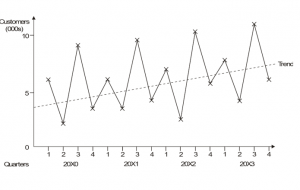
In this example, there would appear to be large seasonal fluctuations in demand, but there is also a basic upward trend.
Cyclical variations
Cyclical variations are medium-term changes in results caused by circumstances which repeat in cycles. In business, cyclical variations are commonly associated with economic cycles, successive booms and slumps in the economy. Economic cycles may last a few years. Cyclical variations are longer term than seasonal variations.
Summarising the components
In practice a time series could incorporate all of the four features we have been looking at and, to make reasonably accurate forecasts, the four features often have to be isolated. We can begin the process of isolating each feature by summarising the components of a time series as follows.
The actual time series, Y= T + S + C + R
where Y = the actual time series C = the cyclical component
T = the trend series R = the random component
S = the seasonal component
Though you should be aware of the cyclical component, it is unlikely that you will be expected to carry out any calculation connected with isolating it. The mathematical models which we will use therefore exclude any reference to C.
We will begin by looking at how to find the trend in a time series.
Moving averages
Trend values can be determined by a process of moving averages.
Look at these monthly sales figures.
August September October November December
Sales 0.02 0.04 0.04 3.20 14.60
(RWFm)
It looks as though the business is expanding rapidly – and so it is, in a way. But when you know that the business is a Christmas card manufacturer, then you see immediately that the January sales will no doubt slump right back down again.
It is obvious that the business will do better in the Christmas season than at any other time – that is the seasonal variation. Using the monthly figures, how can we tell whether or not the business is doing well overall – whether there is a rising sales trend over time other than the short-term rise over Christmas?
One possibility is to compare figures with the equivalent figures of a year ago. However, many things can happen over a year to make such a comparison misleading – new products might now be manufactured and prices will probably have changed.
In fact, there are a number of ways of overcoming this problem of distinguishing trend from seasonal variations. One such method is called moving averages. This method attempts to remove seasonal (or cyclical) variations from a time series by a process of averaging so as to leave a set of figures representing the trend.
A moving average is an average of the results of a fixed number of periods. Since it is an average of several time periods, it is related to the mid-point of the overall period.
Finding the seasonal variations
Seasonal variations can be estimated using the additive model or the proportional (multiplicative) model.
Once a trend has been established we can find the seasonal variations.
The additive model
The additive model for time series analysis is Y = T + S + R.
We can therefore write Y – T = S + R. In other words, if we deduct the trend series from the actual series, we will be left with the seasonal and residual components of the time series. If we assume that the random component is relatively small, and hence negligible, the seasonal component can be found as S = Y – T, the de-trended series.
The proportional model
The method of estimating the seasonal variations in the above example was to use the differences between the trend and actual data. This model assumes that the components of the series are independent of each other, so that an increasing trend does not affect the seasonal variations and make them increase as well, for example.
The alternative is to use the proportional model whereby each actual figure is expressed as a proportion of the trend. Sometimes this method is called the multiplicative model.
The proportional (multiplicative) model summarises a time series as Y = T × S × R.
The trend component will be the same whichever model is used but the values of the seasonal and random components will vary according to the model being applied.
The example above can be reworked on this alternative basis. The trend is calculated in exactly the same way as before but we need a different approach for the seasonal variations. The proportional model is Y = T × S × R and, just as we calculated S = Y – T for the additive model above, we can calculate S = Y/T for the proportional model.
Note that the proportional model is better than the additive model when the trend is increasing or decreasing over time. In such circumstances, seasonal variations are likely to be increasing or decreasing too. The additive model simply adds absolute and unchanging seasonal variations to the trend figures whereas the proportional model, by multiplying increasing or decreasing trend values by a constant seasonal variation factor, takes account of changing seasonal variations.
Time series analysis and forecasting
Forecasts can be made by calculating a trend line (using moving averages or linear regression), using the trend line to forecast future trend line values, and adjusting these values by the average seasonal variation applicable to the future period.
By extrapolating a trend and then adjusting for seasonal variations, forecasts of future values can be made.
Forecasts of future values should be made as follows.
- Find a trend line using moving averages or using linear regression analysis
- Use the trend line to forecast future trend line values.
- Adjust these values by the average seasonal variation applicable to the future period, to determine the forecast for that period. With the additive model, add (or subtract for negative variations) the variation. With the multiplicative model, multiply the trend value by the variation proportion.
Extending a trend line outside the range of known data, in this case forecasting the future from a trend line based on historical data, is known as extrapolation.
Forecasting problems
Errors can be expected in forecasting due to unforeseen changes. This is more likely to happen the further into the future the forecast is for, and the smaller the quantity of data on which the forecast is based.
All forecasts are subject to error, but the likely errors vary from case to case.
- The further into the future the forecast is for, the more unreliable it is likely to be
- The less data available on which to base the forecast, the less reliable the forecast
- The historic pattern of trend and seasonal variations may not continue into the future
- Random variations may upset the pattern of trend and seasonal variation
- Extrapolation of the trend line is done by judgment and can introduce errors
There are a number of changes that also may make it difficult to forecast future events.
| Type of change | Examples |
| Political and economic changes | Changes in interest rates, exchange rates or inflation can mean that future sales and costs are difficult to forecast. |
| Environmental changes | The opening of new roads or the railway might have a considerable impact on some companies’ markets. |
| Technological changes | These may mean that the past is not a reliable indication of likely future events. For example new faster machinery may make it difficult to use current output levels as the basis for forecasting future production output. |
| Technological advances | Advanced manufacturing technology is changing the cost structure of many firms. Improved education and the increase in the standards of living are impacting on the skills of the labour force. This causes forecasting difficulties because of the resulting changes in cost behaviour patterns, breakeven points and so on. |
| Social changes | Alterations in taste, fashion and the social acceptability of products can cause forecasting difficulties. |
Management should have reasonable confidence in their estimates and forecasts. The assumptions on which the forecasts/estimates are based should be properly understood and the methods used to make a forecast or estimate should be in keeping with the nature, quantity and reliability of the data on which the forecast or estimate will be based. There is no point in using a ‘sophisticated’ technique with unreliable data; on the other hand, if there are a lot of accurate data about historical costs, it would be a waste of the data to use the scatter diagram method for cost estimating.
LEARNING CURVES
Learning curve theory may be useful for forecasting production time and labour costs in certain circumstances, although the method has many limitations.
Whenever an individual starts a job which is fairly repetitive in nature, and provided that his speed of working is not dictated to him by the speed of machinery (as it would be on a production line), he is likely to become more confident and knowledgeable about the work as he gains experience, to become more efficient, and to do the work more quickly.
Eventually, however, when he has acquired enough experience, there will be nothing more for him to learn and so the learning process will stop.
Learning curve theory applies to situations where the work force as a whole improves in efficiency with experience. The learning effect or learning curve effect describes the speeding up of a job with repeated performance.
Where does learning curve theory apply?
Labour time should be expected to get shorter, with experience, in the production of items which exhibit any or all of the following features.
- Made largely by labour effort (rather than by a highly mechanised process)
- Brand new or relatively short-lived (learning process does not continue indefinitely)
- Complex and made in small quantities for special orders
The learning rate: cumulative average time
In learning theory the cumulative average time per unit produced is assumed to decrease by a constant percentage every time total output of the product doubles.
For instance, where an 80% learning effect occurs, the cumulative average time required per unit of output is reduced to 80% of the previous cumulative average time when output is doubled.
- By cumulative average time, we mean the average time per unit for all units produced so far, back to and including the first unit made.
- The doubling of output is an important feature of the learning curve measurement.
Don’t worry if this sounds quite hard to grasp in words, because it is hard to grasp (until you’ve learned it!). It is best explained by a numerical example.
A formula for the learning curve
The formula for the learning curve is y = axb, where b, the learning coefficient or learning index, is defined as (log of the learning rate/log of 2).
The formula for the learning curve is y = axb where y is the average cost per batch x is the total number of batches produced a is the cost of the first batch b is the learning factor (logLR/log2)
LR is the learning rate as a decimal
Logarithms and the value of b
When y = axb in learning curve theory, the value of b = log of the learning rate/log of 2. The learning rate is expressed as a proportion, so that for an 80% learning curve, the learning rate is 0.8, and for a 90% learning curve it is 0.9, and so on.
The practical application of learning curve theory
What costs are affected by the learning curve?
- Direct labour time and costs
- Variable overhead costs, if they vary with direct labour hours worked.
- Materials costs are usually unaffected by learning among the workforce, although it is conceivable that materials handling might improve, and so wastage costs be reduced.
- Fixed overhead expenditure should be unaffected by the learning curve (although in an organisation that uses absorption costing, if fewer hours are worked in producing a unit of output, and the factory operates at full capacity, the fixed overheads recovered or absorbed per unit in the cost of the output will decline as more and more units are made).
The relevance of learning curve effects in management accounting
Learning curve theory can be used to:
- Calculate the marginal (incremental) cost of making extra units of a product.
- Quote selling prices for a contract, where prices are calculated at cost plus a percentage mark-up for profit. An awareness of the learning curve can make all the difference between winning contracts and losing them, or between making profits and selling at a loss-making price.
- Prepare realistic production budgets and more efficient production schedules.
- Prepare realistic standard costs for cost control purposes.
Considerations to bear in mind include:
- Sales projections, advertising expenditure and delivery date commitments. Identifying a learning curve effect should allow an organisation to plan its advertising and delivery schedules to coincide with expected production schedules. Production capacity obviously affects sales capacity and sales projections.
- Budgeting with standard costs. Companies that use standard costing for much of their production output cannot apply standard times to output where a learning effect is taking place. This problem can be overcome in practice by:
- Establishing standard times for output, once the learning effect has worn off or become insignificant, and
- Introducing a ‘launch cost’ budget for the product for the duration of the learning period.
- Budgetary control. When learning is still taking place, it would be unreasonable to compare actual times with the standard times that ought eventually to be achieved when the learning effect wears off. Allowance should be made accordingly when interpreting labour efficiency variances.
- Cash budgets. Since the learning effect reduces unit variable costs as more units are produced, it should be allowed for in cash flow projections.
- Work scheduling and overtime decisions. To take full advantage of the learning effect, idle production time should be avoided and work scheduling/overtime decisions should pay regard to the expected learning effect.
- Pay. Where the workforce is paid a productivity bonus, the time needed to learn a new production process should be allowed for in calculating the bonus for a period.
- Recruiting new labour. When a company plans to take on new labour to help with increasing production, the learning curve assumption will have to be reviewed.
- Market share. The significance of the learning curve is that by increasing its share of the market, a company can benefit from shop-floor, managerial and technological ‘learning’ to achieve economies of scale.
Limitations of learning curve theory
- The learning curve phenomenon is not always present.
- It assumes stable conditions at work which will enable learning to take place. This is not always practicable, for example because of labour turnover.
- It must also assume a certain degree of motivation amongst employees.
- Breaks between repeating the production of an item must not be too long, or workers will ‘forget’ and the learning process will have to begin all over again.
- It might be difficult to obtain accurate data to decide what the learning curve is.
- Workers might not agree to a gradual reduction in production times per unit.
- Production techniques might change, or product design alterations might be made, so that it takes a long time for a ‘standard’ production method to emerge, to which a learning effect will apply.
APPLYING EXPECTED VALUES
Expected values can be used in budgeting to determine the best combination of expected profit and risk.
Probabilistic budgeting assigns probabilities to different conditions (most likely, worst possible, best possible) to derive an Expected Value (EV) of profit.
USING SPREADSHEETS IN BUDGETING
Spreadsheet packages can be used to build business models to assist the forecasting and planning process. They are particularly useful for ‘what if?’ analysis.
A spreadsheet is a type of general purpose software package with many business applications, not just accounting ones. It can be used to build a model, in which data is presented in these rows and columns, and it is up to the model builder to determine what data or information should be presented in it, how it should be presented and how the data should be manipulated by the spreadsheet program. The most widely used spreadsheet packages are IBM Lotus 1-2-3 and Microsoft Excel.
The idea behind a spreadsheet is that the model builder should construct a model as follows.
- Identify what data you have and what you want to report.
- Then decide what data go into each row and column and by inserting text (for example, column headings and row identifications).
- Specify how the numerical data in the model should be derived. Numerical data might be derived using one of the following methods.
- Insertion into the model via keyboard input.
- Calculation from other data in the model by means of formulae specified within the model itself. The model builder must insert these formulae into the spreadsheet model when it is first constructed.
- Retrieval from data on a disk file from another computer application program or module.
The advantages of spreadsheets
The uses of spreadsheets are really only limited by your imagination, and by the number of rows and columns in the spreadsheet, but some of the more common accounting applications are listed below.
- Balance sheets Profit projections
- Cash flow analysis/forecasting Profit statements
- General ledger Project budgeting and control
- Inventory records Sales projections and records
- Job cost estimates Tax estimation
- Market share analysis and planning
The great value of spreadsheets derives from their simple format of rows, columns and worksheets of data, and the ability of the data users to have direct access themselves to their spreadsheet model via their own PC. For example, an accountant can construct a cash flow model with a spreadsheet package on the PC on his desk: he can create the model, input the data, manipulate the data and read or print the output direct. He will also have fairly instant access to the model whenever it is needed, in just the time it takes to load the model into his PC. Spreadsheets therefore bring computer modelling within the everyday reach of data users.
Also, by linking different models, when one spreadsheet is updated say for Sales, another such as Raw material stocks can be updated as well – automatically
The disadvantages of spreadsheets
Spreadsheets have disadvantages if they are not properly used.
- A minor error in the design of a model at any point can affect the validity of data throughout the spreadsheet. Such errors can be very difficult to trace.
- Even if it is properly designed in the first place, it is very easy to corrupt a model by accidentally changing a cell or inputting data in the wrong place. This can be minimised by “protecting” cells containing formulae or fixed data
- It is possible to become over-dependent on them, so that simple one-off tasks that can be done in seconds with a pen and paper are done on a spreadsheet instead.
- The possibility for experimentation with data is so great that it is possible to lose sight of the original intention of the spreadsheet.
- Spreadsheets cannot take account of qualitative factors since these are invariably difficult to quantify. Decisions should not be made on the basis of quantitative information alone.
In summary, spreadsheets should be seen as a tool in planning and decision making. The user must make the decision.
CHAPTER ROUNDUP
- Two important quantitative methods the management accountant can use to analyse fixed and variable cost elements from total cost data are the high-low and regression methods.
- Scatter diagrams can be used to estimate the fixed and variable components of costs.
- Forecasting techniques include estimates based on judgement and experience, simple average growth models and time series.
- A time series is a series of figures or values recorded over time.
- Regression can be used to find a trend line, such as the trend in sales over a number of periods.
- A time series has four components: a trend, seasonal variations, cyclical variations and random variations.
- Trend values can be determined by a process of moving averages.
- Seasonal variations can be estimated using the additive model or the proportional (multiplicative) model.
- Forecasts can be made by calculating a trend line (using moving averages or linear regression), using the trend line to forecast future trend line values, and adjusting these values by the average seasonal variation applicable to the future period.
- Errors can be expected in forecasting due to unforeseen changes. This is more likely to happen the further into the future the forecast is for, and the smaller the quantity of data on which the forecast is based.
- Learning curve theory may be useful for forecasting production time and labour costs in certain circumstances, although the method has many limitations.
- The formula for the learning curve is y = axb, where b, the learning coefficient or learning index, is defined as (log of the learning rate/log of 2).
- Expected values can be used in budgeting to determine the best combination of expected profit and risk.
- Spreadsheet packages can be used to build business models to assist the forecasting and planning process. They are particularly useful for ‘what if?’ analysis.