
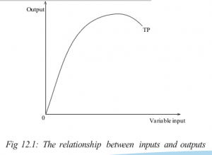
Production function is an expression of the relationship between physical quantities of inputs and output. It shows the maximum output that can be obtained from a given quantity of physical inputs.
- As a statement Q = f(L,K,N,M,T).
The relationship can be expressed mathematically as follows:
Q= f (L, K, N, M, T). Where Q is output, K is capital, N is land, M is organisation, T is technology and L is labour. f stands for function. The left hand side (Q) represents the dependent variable while the right hand side represents the independent variables. Thus output is the dependent variable while input is the independent variable.
- As an equation Y = a + bx.
Where Y is output, a and b are constants and x is variable input.
- As a graph.
Using a graph, it can be represented as follows:
The above mentioned are forms in which the production function can be expressed. However, it is important to note that the standard economic assumption, which affects the shape of the production function, is the law of diminishing returns.
12.1.2: The law of diminishing returns and returns to scale
(b) In your groups discuss the laws of diminishing returns and returns to scale, their assumptions and illustrations. Make presentations in class.
The law of diminishing returns states that “ As more of a variable input X is added to a fixed factor, total output increases at an increasing rate and later decreases at a decreasing rate until a point is reached where additional quantities of input X will yield diminishing marginal returns, assuming all other factors remain constant.” This law is also called the law of variable proportions.
12.1.2.1 Assumptions of the law of diminishing returns
- Existence of a variable factor of production and other factors are constant.
- All units of the variable factor are homogeneous.
- The price of the product is given and constant.
- It assumes a short run period.
- It is possible to change the proportions in which various inputs are combined.
It assumes that technology is constant.
12.1.3: The law of returns to scale
The law of returns to scale is an expression of the relationship between output and the scale of inputs in the long run when all inputs are increased in the same proportion. Returns to scale, in physical or money terms can be of three types:
- Constant returns to scale: This is a situation where an increase in inputs results in an exactly proportional increase in output.
| Capital (K) | Labour (L) | Output |
| 2 | 2 | 3 |
| 4 | 4 | 6 |
| 8 | 8 | 12 |
Under constant returns to scale, when inputs double, output also doubles.
- Increasing returns to scale: This is a situation where an increase in inputs results in a more than proportional increase in output.
| Capital (K) | Labour (L) | Output |
| 2 | 2 | 3 |
| 4 | 4 | 7 |
| 8 | 8 | 16 |
Under increasing returns to scale, when inputs double, output more than doubles.
-
Capital (K) Labour (L) Output 2 2 3 4 4 5 8 8 8 Decreasing returns to scale: This is a situation where an increase in inputs results in a less than proportional increase in output.
Under decreasing returns to scale, when inputs double, output less than doubles. Output increases at a decreasing rate.
12.1.3.1 Assumptions of the law
- It assumes that all factors are variable.
- It assumes constant technology. iii) It assumes that the product can be measured in physical quantities. iv) It assumes perfect competition conditions.
12.1.4: The products of the firm
12.1.4.1 Total product
This refers to total output resulting from the employment of all the factors of production.
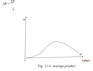
Average product (AP)
This is the output per unit of a variable factor employed. It is the total product divided by the total units of a variable factor. As more of a variable factor is employed, AP increases fast, then it falls and the point where AP is at maximum is referred to as the point of diminishing average productivity.
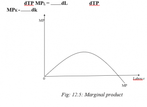
Marginal product (MP)
This is the additional output produced by an extra unit of a variable factor. It is the change in total product as a result of a unit change in the variable factor. It is that output that results from employment of an addition of a variable factor.
Production function MP & AP schedule
| Labour (L)
|
Total product
(Q) |
Average product
(AP) |
Marginal product
(MP) |
| 1 | 10 | 10 | – |
| 2 | 22 | 11 | 12 |
| 3 | 36 | 12 | 14 |
| 4 | 48 | 12 | 12 |
| 5 | 55 | 11 | 7 |
| 6 | 60 | 10 | 5 |
| 7 | 60 | 8.6 | 0 |
| 8 | 56 | 7 | -4 |
The table above shows the variable factor labour being combined with fixed factor land and the resultant output is obtained. The production function is revealed in the first two columns i.e. (1) and (2). The AP and MP columns are derived from the total product column. The AP is obtained by dividing column (2) by a corresponding unit in column (1). The MP is the addition to total product by an extra worker.
12.1.4.5 The relationship between TP, MP and AP
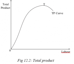
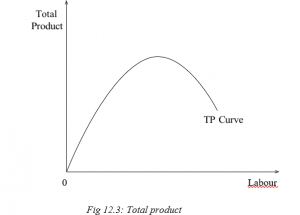
The analysis of the table shows that the total, average and marginal product increase at first, reach a maximum and then start declining. The TP reaches its maximum when 6 units of labour are employed and it declines. The AP continues to rise till the 4th unit while the MP reaches its maximum at the 3rd unit of labour, then they also fall.
Note: The point of falling output is not the same for total, average and marginal product curves. The MP starts declining first, then AP follows and lastly, the total product (TP).
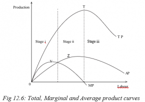
The TP curve rises at an increasing rate up to its highest point T and then starts falling. The MP curve and the AP also rise with the total product.
The MP reaches its maximum point V and declines while the AP reaches its maximum point Z and starts falling. When the TP starts declining, the MP curve becomes negative. It is only when the TP is zero that the average product also becomes zero.
The rising, falling and negative phases of the TP, MP and AP are the different stages of the law of variable proportions. The boundary between stage II and III shows the level at which all resources are fully utilised. However, it would be irrational to limit production to stage I because a variable input will not be fully utilised for example the AP is still increasing.
In stage III it is rational to limit operation because you cannot continue adding an input when the TP is decreasing and the MP is negative, unless the input is bought at a negative cost. It is also irrational to continue adding variable inputs when fixed inputs are fully utilised. Therefore the best stage of production is stage II. It is the only stage when production is feasible and profitable.
12.2: ISOQUANTS AND ISOCOSTS
12.2.1: Isoquants
Activity 12.6
- Below is a table showing how a firm can vary units of capital and labour to produce the same level of output of 200 units
Combination Units of capital Units of labour Total output
- 10 5 200
- 7 10 200
- 4 15 200
- 2 20 200
Given that the producer’s income to spend on capital and labour is FRW 200,000.
In groups of five, represent the above data on a graph. Discuss the properties of the graph. Make a presentation in class.
Facts
An isoquant is a locus of points joining different input combinations, capable of producing the same level of output. An isoquant is also referred to as the production indifference curve. The slope of an isoquant is known as the marginal rate of technical substitution since it shows the rate at which one input is substituted for another while maintaining the same level of output. It can be illustrated from the hypothetical isoquant schedule below.
12.2.1.1 Hypothetical isoquant schedule
| Combination | Units of capital | Units of labour | Total output |
| A | 10 | 4 | 100 |
| B | 8 | 9 | 100 |
| C | 6 | 14 | 100 |
| D | 4 | 19 | 100 |
The table shows that a firm can produce 100 units of output at point A by having a combination of 10 units of capital and 4 units of labour. Similarly point B shows a combination of 8 units of capital and 9 units of labour. Point C, 6 units of capital and 14 units of labour and point D, 4 units of capital and 19 units of labour to yield the same amount of 100 units.
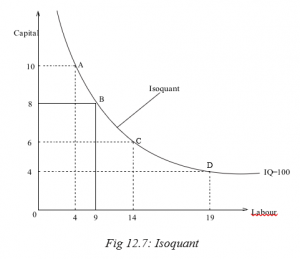
When labour units are measured along the X- axis and capital units along the Y- axis, the first, second, third and fourth combinations are shown as A, B, C and D respectively. When we connect all these points, we get the isoquant curve.
12.2.1.2 Properties of isoquants
Isoquants possess certain characteristics, which are similar to those of indifference curves:
- Isoquants are negatively inclined. That is to say as the amount of capital decreases, that of labour increases so that output remains constant.
- An isoquant lying above and to the right of another represents a higher output level.
- No two isoquants can intersect each other, that is, the point of intersection combination would bear less and more output at the same time which is not possible.
- In between two isoquants, there can be a number of isoquants showing various levels of output.
- No isoquant can touch either axis. If an isoquant touches the X- axis, it would mean that the product is being produced with the help of labour alone without using any capital.
- Each isoquant is convex to the origin. As more units of labour are employed to produce 100 units of a product, lesser and lesser units of capital are used. This is because the marginal rate of substitution between the two factors diminishes.
12.2.2: Isocosts
An isocost is a line of points joining different input combinations, which exhaust the producer’s income. It represents the different combinations of two inputs that a firm can buy for a given sum of money at the given price of each input. Isocosts are straight lines because factor prices remain the same whatever the outlay of the firm on the two factors.
Hypothetical table
Isocost curve
The Isocost curve represents the locus of all combinations of the two factor inputs which result from the same total cost. If for example the unit cost of labour (L) is w and the unit cost of capital (k) is r, then the total cost is:
Total cost =wL + rK
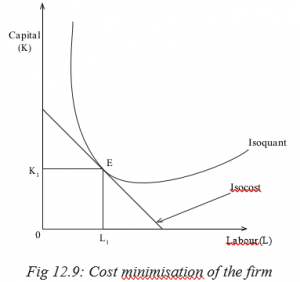
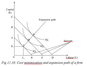
The firm will be in equilibrium when the highest isoquant curve becomes tangent to the isocost line. At point E, the equilibrium position of the firm is defined as the level of maximum output, subject to the cost constraint. This point is always shown where the isoquant curve is tangent to the isocost. The point of tangency represents the least cost combination of the two factors for producing a given output.
Remember!!! Producers should not compromise standard and quality of goods as they try to increase the firm’s product.
If all points of tangency like L, M and N are joined by a line, that ‘joining’ line is known as the expansion path or the output factor curve. It shows how the proportions of the two factors used might be changed as the firm expands.
Unit Summary
The unit discussed:
- The production functions as the expression of the relationship between output and inputs.
- The planning periods, that is, the short run period as the period during which some factors of production are variable while others are fixed; and long run period as the period when all factors of production are variable.
- Products of the firm were also discussed. Total product is the total amount of goods produced by the firm, average product is the output per unit of the variable factor and marginal product is the additional output got by employing an extra unit of a variable factor.
Unit Assessment 12
- (a) What is meant by the production function?
- Describe the different forms in which the production function can be expressed.
- (a) Define the terms total product, average product and marginal
- Explain the relationship between total product, average product and marginal product.
- (a) State the law of diminishing returns.
- List the assumptions of the law of diminishing returns.
- (a) State the law of returns to scale
(b) Distinguish between constant returns to scale, increasing returns to scale and decreasing returns to scale.
5 (a) Distinguish between an isoquant and an isocost.
(b) Explain the properties of isoquants.