
We can use simple algebra to determine national income. National income is at equilibrium when Ag. Demand equals Ag. Supply. In a simple closed model of income determination without gov. expenditure, taxation, then
Y=C+I
Suppose the consumption function is of the form:
C=a+bY suppose investment demand equals I0 (Autonomous)
We get the following 3 equations for the determination of equilibrium level of national income.
Y=C+I
C=a+bY
I=I0
Substitute C and I in the first equation we have: Y=a+bY+I0
Y-bY=a+I0
Y(1-b)=a+I0
Y=1/1-b (a+I0)
The last equation shows the equilibrium level of national income when ag. Demand equals. Ag. Supply. Equilibrium level of income can be known by multiplying the sum of autonomous consumption and expenditure with the multiplier Suppose an economy has autonomous investment of 600 and the consumption function is given by C=200+0.8Y. Find equilibrium level of income The issues of consumption investment and savings will be explored further in the subsequent lecture.
3.2 Consumption, Investment, Savings and Tax Functions
Consumption and Savings
We assume a closed economy that has three uses for the goods and services it produces. These three components of GDP are expressed in the national income accounts identity as:
Y = C + I + G
Households consume some of the economy‘s output; firms and households use some of the output for investments; and the government buys some of the output for public purposes. Aggregate demand is the total amount of goods demanded in the economy. Output is at equilibrium when the quantity of output produced is equal to the quantity demanded. Thus, the national accounts identity can be expressed as:
AD = Y= C+I+G
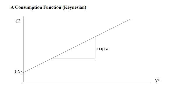
In practice the demand for consumption goods increases with income. The relationship between consumption and income is described by the consumption function. Households receive income from their labor and their ownership of capital, pay taxes to the government, and then decide how much of their after tax income they will consume and how much to save. Assuming that households receive income equal to the output of the economy Y and that the government then taxes the households an amount T, we can define income after taxes (Y-T), as disposable income. Households divide their disposable income between consumption and savings. We assume that the level of consumption is directly depends on the level of disposable income. The higher is the disposable income, the greater is consumption. Thus
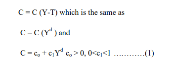
The variable co, the intercept, represents the level of consumption when income is zero. The coefficient c1 is known as the marginal propensity to consume. It measures the amount by which consumption changes when income increases by one shilling. In our case, the marginal propensity to consume is less than one, which implies that out of a shilling increase in income, only a fraction, c1 is spent.
After a household spends in consumption what remains must be saved. More formally saving is equal to income minus consumption. Thus S = Yd-C
The savings function relates to the level of income. Substituting the consumption function in equation one we get a savings function as follows:
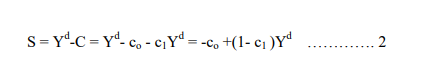
From equation 2 we see that saving is an increasing function of the level of income because the marginal propensity to save, s= (1- c1 ), is positive. In other words, savings increases as income rises. For instance, suppose the marginal propensity to consume is 0.8, meaning that 80 cents out of each extra shilling of income is consumed. Then the marginal propensity to save s, is 0.2, meaning that the remaining 20 cents of each extra shilling of income is saved.
Taxes
Taxes play a major role in financing government expenditure. We shall now analyze the effects of taxes on the equilibrium level of income keeping gov. expenditure constant. Simplest kind of tax is the lumpsum tax in which a given amount of revenue is collected
irrespective of the level of income. After taxes people consume less and save less. However consumption will not fall by the full amount of taxes.
This is because part of the disposable income was being consumed and part was being saved prior to taxation. Hence the decline disposable income due to the lumpsum tax will partly cause a decline in consumption and savings. Consumption will fall by the amount of tax multiplied my MPC. If Yd is change in disposable income, T for tax, then the decline in consumption (-ΔC)is given by
-ΔC=T.MPC
Since T= ΔYd
-ΔC=ΔYd.MPC
For example:
Suppose government imposed 500 lumpsum tax. The MPC is 0.75 then decline in consumption
is 500 X 0.75=375.
If taxes were reduced consumption will increase by the amount of lumpsum tax multiplied by
MPC ie +ΔC=ΔYd.MPC. Impositions of Taxes shift the consumption function downwards while a reduction in taxes shifts consumption function upwards. A fall in NI after imposition of taxes is not equal to the amount of tax collected, but by a multiplier of it. The multiplier is equal to: -b/1- b where b is the MPC. This is called the tax multiplier
Investment
Both firms and households purchase investment goods, Firms buy investment goods to add to their stock of capital and to replace existing capital as it wears out. Households buy new houses, which are also part of investment. The quantity of investment goods demanded depends on interest rate, which measures the cost of the funds used to finance investment. We can distinguish between nominal interest rate, which is interest rate as usually reported, and the real interest rate, which is the nominal interest rate corrected for the effects of inflation. If the nominal interest rate is 10 percent and the inflation rate is 3 percent, then the real interest rate is
7 percent. Here it is important to note that the real interest rate measures the cost of borrowing, and thus determines the quantity of investment.
Thus I = I(r)
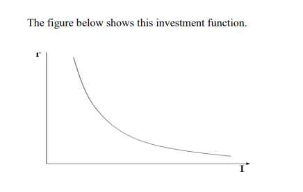
Investment function 1
The investment function slopes downwards, because as the interest rate rises, the quantity of investment demanded falls.
Government Purchases
The government purchases are a third component of the demand for goods and services. The governments buys guns, build roads and other public works. It also pays salaries to civil servants. If government purchases equal taxes then the government has a balanced budget. If G exceeds T then the government runs into a budget deficit. If G is less than T then the government runs a budget surplus. For our discussion we take Government purchases and taxes as exogenous variables.
Thus G = Go
T = To
3.3 Determination of Equilibrium National Income
Using the above information we can obtain equilibrium in two ways
- Using goods market and service market
- Financial markets
Equilibrium in the market for goods and services
Using the relationships discussed above we can get the equilibrium level of income or output as follow:
Y = C + I + G
C = co + c1Y
d
I = I (r)
G = Go
T = To
We can combine these equations to obtain equilibrium level of income.
Y = co + c1 (Y-To) + I(r) + Go
The above model of income determination is known as the Keynesian model of income determination.
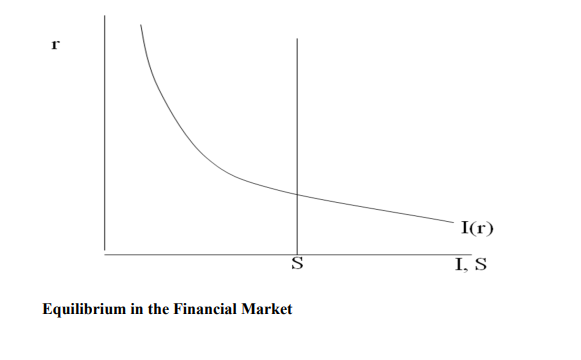
Equilibrium in the Financial Markets
To obtain equilibrium in the financial markets, we consider savings and investment. Savings represent the supply of supply of loanable funds while investment represents demand for loanable funds .We can be able to analyze the financial markets by examining the interest rate, which is the cost of borrowing and the return to lending in the financial markets. We can rewrite the national income identity
Y = C + I + G as Y-C-G = I
The term on the left hand side is the output that remains after the demands of consumers and the government has been satisfied. It is called national saving. In this form the national income accounts identity shows that saving equal investment. Savings represent the supply of loanable funds while investment represents the demand for these funds. The quantity of investment demanded will depend on the cost of borrowing. At equilibrium interest rate the households‘ desire to save balances firms‘ desire to invest and the quantity of loans supplied equals the quantity demanded.
The Expenditure Multiplier
This is the amount by which equilibrium output changes when autonomous aggregate demand increases by one unit. Assuming the absence of the government and foreign sector the multiplier is defined as
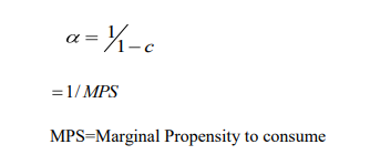
From the above equation you observe that the larger the marginal propensity to consume the larger the multiplier. The multiplier suggests that output changes when autonomous spending changes and that the change in output can be larger than the change in autonomous spending.