
INTRODUCTION
As we saw earlier in this study unit, costs can be divided either into direct and indirect costs, or variable and fixed costs.
Direct costs are variable, that is the total cost varies in direct proportion to output. If, for instance, it requires RWF10 worth of material to make one item it will require RWF20 worth to make two items and RWF100 worth to make ten items and so on.
Overhead costs, however, may be either fixed, variable or semi-variable.
FIXED COST
A fixed cost is one which can vary with the passage of time but, within limits, tends to remain fixed irrespective of the variations in the level of output. All fixed costs are overhead. Examples of fixed overhead are: executive salaries, rent, rates and depreciation.
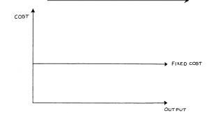
Please note the words “within limits” in the above description of fixed costs. Sometimes this is referred to as the “relevant range”, that is the range of activity level within which fixed costs (and variable costs) behave in a linear fashion.
Suppose an organisation rents a factory. The yearly rent is the same no matter what the output of the factory is. If business expands sufficiently, however, it may be that a second factory is required and a large increase in rent will follow. Fixed costs would then be as in Figure 5.
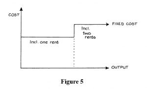
A cost with this type of graph is known as a step function cost for obvious reasons.
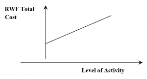
VARIABLE COST
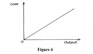
This is a cost which tends to follow (in the short term) the level of activity in a business.
As already stated, direct costs are by their nature variable. Examples of variable overhead are: repairs and maintenance of machinery; electric power used in the factory; consumable stores used in the factory.
The graph of a variable cost is shown in Figure 6.
SEMI-VARIABLE (OR SEMI-FIXED) COST
This is a cost containing both fixed and variable elements, and which is thus partly affected by fluctuations in the level of activity.
For examination purposes, semi-variable costs usually have to be separated into their fixed and variable components. This can be done if data is given for two different levels of output.
STEP COST
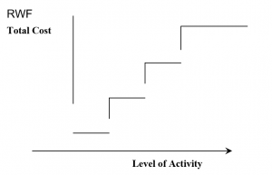
Rent can be a step cost in certain situations where accommodation requirements increase as output levels get higher.
A Step Cost
Many items of cost are a fixed cost in nature within certain levels of activity.
Semi-Variable Costs
This is a cost containing both fixed and variable components and which is thus partly affected by fluctuations in the level of activity (CIMA official DFN).
Example: Running a Car
- Fixed Cost is Road Tax and insurance.
- Variable cost is petrol, repairs, oil, tyres-all of these depend on the number of miles travelled throughout the year.
High – Low method
Firstly, examine records of cost from previous period. Then pick a period with the highest activity level and the period with the lowest level of activity.
- Total Cost of high activity level minus total cost of low activity level will equal variable cost of difference in activity levels.
Fixed Costs are determined by substitution
Scattergraphs
Information about two variables that are considered to be related in some way can be plotted on a scattergraph. This is simply a graph on which historical data can be plotted. For cost behaviour analysis, the scattergraph would be used to record cost against output level for a large number of recorded “pairs” of data.
Then by plotting cost level against activity level on a scattergraph, the shape of the resulting figure might indicate whether or not a relationship exists.
In such a scattergraph, the y axis represents cost and the x axis represents the output or activity level.
One advantage of the scattergraph is that it is possible to see quite easily if the points indicate that a relationship exists between the variables, i.e. to see if any correlation exists between them.
Positive correlation exists where the values of the variables increase together (for example, when the volume of output increases, total costs increase).
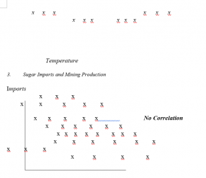
Negative correlation exists where one variable increases and the other decreases in value Some illustrations:
- Weight and height in humans
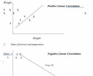
A scattergraph can be used to make an estimate of fixed and variable costs, by drawing a “line of best fit” through the band of points on the scattergraph, which best represents all the plotted points.
The above diagrams contain the line of best fit. These lines have been drawn using judgement. This is a major disadvantage, as drawing the line “by eye”. If there is a large amount of scatter, different people may draw different lines.
Thus, as a technique, it is only suitable where the amount of scatter is small or where the degree of accuracy of the prediction is not critical.
However, it does have an advantage over the high-low method in that all points on the graph are considered, not just the high and low point.
Regression Analysis
This is a technically superior way to identify the “slope” of the line. It is also known as “Least Squares Regression”. This statistical method is used to predict a linear relationship between two variables. It uses all past data (not just the high and low points) to calculate the line of best fit.
THE LINEAR ASSUMPTION OF COST BEHAVIOUR
- Cost are assumed to be either fixed, variable or semi-variable within a normal range of output.
- Fixed and variable costs can be estimated with degrees of probable accuracy. Certain methods maybe used to access this (High-Low method).
- Costs will rise in a straight line/linear fashion as the activity increases.
ACCOUNTANTS – V’S – ECONOMIST MODEL
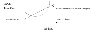
Assumptions of Above Diagram
The accountants state that the linear assumption of cost behaviour is linear because:
- The linear cost (straight line) is only used in practice within normal ranges of output [ ‘Relevant Range of Activity’.
The term ‘Relevant Range’ is used to refer to the output range at which the firm expects to be operating in the future.
- It is easier to understand than Economists’ cost line.
- The fixed and variable costs are easier to use.
- The relevant range and the costs estimated by the economists and the accountants will not be very different.
FACTORS AFFECTING THE ACTIVITY LEVEL
- The economic environment.
- The individual firm – its staff, their motivation and industrial relations.
- The ability and talent of management.
- The workforce (unskilled, semi-skilled and highly skilled).
- The capacity of machines.
- The availability of raw material.
COST BEHAVIOUR AND DECISION MAKING
Factors to Consider:
- Future plans for the company.
- Current competition to the company.
- Should the selling price of a single unit be reduced in order to attract more customers.
- Should sale staff be on a fixed salary or on a basic wage with bonus/commission.
- Is a new machine required for current year.
- Will the company make the product internally or buy it.
For all of the above factors, management must estimate costs at all levels and evaluate different courses of action. Management must take all eventualities into account when making decisions for the company.
Example of things management would need to know is fixed costs do not generally change as a result of a decision unless the company have to rent an additional building for a new job etc.
COST VARIABILITY AND INFLATION
Care must be taken in interpreting cost data over a period of time if there is inflation. It may appear that costs have risen relative to output, but this may be purely because of inflation rather than because the amount of resources used has increased.
If a cost index, such as the Retail Price Index, is available the effects of inflation can be eliminated and the true cost behaviour pattern revealed.
It is essential for the index selected to be relevant to the company; if one of the many Central Statistical Office indices is not appropriate, it may be possible for the company to construct one from its own data.
Consider the following example, which deals with the relationship between production output and the total costs of a single-product company, taken over a period of four years:
Limitations
This forecast of RWF26,250 for the total costs in Year 5 is, of course, subject to many limitations. The method of calculation assumes that all costs are either absolutely fixed or are variable in direct proportion to the volume of production. In practice, as we have seen, it is usually found that “fixed” costs will tend to rise slightly in steps, while the variable costs will usually rise less steeply at the higher levels of output, because of the economies of scale.
Also, our forecast will only be as accurate as our forecast of the cost index for Year 5. This is as difficult to predict as the Retail Price Index, which is influenced by changes in the price of each item in the “shopping basket”.
The analysis of cost behaviour in this way is thus useful as a guide to management, provided we remember that:
- It assumes a linear (or “straight line”) relationship between volume and cost.
- Costs will be influenced by many other factors, such as new production methods or new plant.
- Inflation will have a varying effect on different items of cost.
This subject of cost behaviour is fundamental to many aspects of cost accounting.