
 UNIVERSITY EXAMINATIONS: 2014/2015
ORDINARY EXAMINATION FOR THE BACHELOR OF SCIENCE
IN INFORMATION TECHNOLOGY/BACHELOR OF
INFORMATION TECHNOLOGY
BIT 2304 COMPUTER GRAPHICS
DATE: APRIL, 2015 TIME: 2 HOURS
INSTRUCTIONS: Answer Question ONE and any other TWO
QUESTION ONE (30 MARKS)
a) The most popular technique used in computer animation is the key frame
interpolation technique or in-betweening.
Consider an object with its local origin at an initial position Pin = (Xin,Yin,Zin) at key
frame KFin, which then attains the final position of Pfin =(Xfin, Yfin’ Zfin) at keyframe
KFfin.
Now suppose we needed two in-between frames, Fi and Fj
.
Determine the coordinates of the two in- between frames.
(15 Marks)
b) Figure 1 below, shows a ball, initially at position A, with its origin located at
(O,A,O). It falls to the ground at position B, which sets the ball’s origin to (O,B,O).
The ball finally bounces back to position C, which is lower than position A, and the
ball’s origin is at (O,C,O).
The ball moves vertically (Ty along the Y axis) and its movement is graphically
represented in the accompanying graph shown below. The vertical axis of the graph is
the y-displacement of the ball and the horizontal axis is the time axis. The graph also
shows where the ball actually is in the display window in the three key frames.
Let us say we want this animation to be 20 frames long, with the ball starting at frame
1 at position A, reaching position B at frame 10, and reaching position C at frame 20.
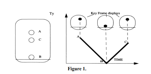
Figure 1.
Determine the positions of the ball in the intermediate frames. (Assume that the ball
does not move in the X and Z axis, thus the motion along these axes will always remain
zero) . (15 Marks)
QUESTION TWO (20 MARKS)
Geometric transformations like rotation, translation, scaling, and projection can be
accomplished with matrix multiplication, and the transformation matrices.
a) OUTLINE the linear 3D transformation matrix describing each of the following.
i) Rotation
ii) Scaling
iii) Translation
iv) Shearing (10 Marks)
b)DESCRIBE in words what this 2D transform matrix does:
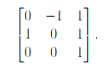
5 Marks)
c) DETERMINE the 3×3 matrix that rotates a 2D point by angle θ about a point p =
(xp,yp).
(5 Marks)
QUESTION THREE (20 MARKS)
Using Figures and/or diagrams , EXPLAIN the following concepts as relates to computer
graphics;
i) Vector Refresh Display
ii) Raster Refresh Display
iii) Scan Conversion
iv) Antialiasing
v) Computer Graphics Pipeline (4 Marks Each)
QUESTION FOUR (20 MARKS)
Using the Raster Image below (Figure 2), explain the concept behind Run-Length
RLE
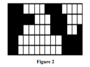
Encoding technique.
4.2.1 Run length encoding
One of the most common and simplest techniques for reducing the data volume
associated with a raster image is a technique known as run length encoding. This
technique reduces the information stored for each line in a raster matrix by storing a single
value for the consecutive number of cells of a given type, rather than storing a value for
each cell. Consider the following simple raster in Figure 9 showing the presence or
absence of clay.
A run length encoded version of the file would be represented as follows:
If we take a closer look at the first row of the run length encoded file we can see how the
method works:
31, 40, 31, 40
The first number (3) represents the number of consecutive cells with the same coding. In
this case the coding 1 = soil type A (clay soil). The third number (4) indicates the number
of unoccupied cells moving from left to right. The fourth number (0) represents the
absence of clay soil. The fifth number (3) denotes the next 3 consecutive cells are
occupied by clay soil (code = 1 again). Finally, the numbers 4 and 0 indicate the absence
of clay soil in the 4 grid cells that complete the row. Note that the commas have been
added to make the file easier to read – they would be absent in a real run length encoded
file e.g. 31403140
If we assume one numeric value uses one byte of storage (1 byte = 8 bits) on the
computer then row one of our run length encoded (RLE) file takes up 8 bytes compared
with the 14 bytes required to store the same information using the simple raster data
structure. The equivalent file sizes and savings are given below:
4.2.1 Run length encoding
One of the most common and simplest techniques for reducing the data volume
associated with a raster image is a technique known as run length encoding. This
technique reduces the information stored for each line in a raster matrix by storing a single
value for the consecutive number of cells of a given type, rather than storing a value for
each cell. Consider the following simple raster in Figure 9 showing the presence or
absence of clay.
Figure 9. Simple raster file structure.
A run length encoded version of the file would be represented as follows:
If we take a closer look at the first row of the run length encoded file we can see how the
method works:
The first number (3) represents the number of consecutive cells with the same coding. In
this case the coding 1 = soil type A (clay soil). The third number (4) indicates the number
of unoccupied cells moving from left to right. The fourth number (0) represents the
absence of clay soil. The fifth number (3) denotes the next 3 consecutive cells are
occupied by clay soil (code = 1 again). Finally, the numbers 4 and 0 indicate the absence
of clay soil in the 4 grid cells that complete the row. Note that the commas have been
added to make the file easier to read – they would be absent in a real run length encoded
file e.g. 31403140
If we assume one numeric value uses one byte of storage (1 byte = 8 bits) on the
computer then row one of our run length encoded (RLE) file takes up 8 bytes compared
with the 14 bytes required to store the same information using the simple raster data
structure. The equivalent file sizes and savings are given below:
BYTE storage requirements
Simple raster Run length raster
Saving 38 bytes 46% saving in
storage space
The figure below shows how the data volume associated with the storage of a complex
raster using the RLE method could be reduced in a similar way. Note that the presence or
absence values of 0 and 1 have been extended to include the codes used to identify 3
different soil types present in the grid.
Figure 10 Complex raster file structure.
An RLE version of the complex raster file would be represented as follows:
As Peuquet (1990) points out, the advantages of the raster spatial data model that
employs a square tessellation is that each cell can be subdivided into smaller cells of the
same shape and orientation. This unique feature of the grid or raster data model has
produced a range of innovative data storage and data reduction methods that are based
on a regularly subdividing geographical space. The most widely implemented is the
Figure 2
(20 Marks)
QUESTION FIVE (20 MARKS)
List and discuss the various ways that 3D models can be created in computer graphics.
(20 Marks)