
7.1 THE EFFECTS OF A SHIFT INAGGREGATE DEMAND
Suppose that for some reason a wave of pessimism suddenly overtakes the economy. The cause might be a government scandal, a crash in the stock market or the outbreak of war overseas. because of this event; many people lose confidence in the future and alter their plans. Household cut back on their spending and delay major purchases and firms put off buying new equipment.
The impact of this is the reduction of the aggregate demand for goods and services. That is, for any given price level, households and firms now want to buy a smaller quantity of goods and services.
The figure below shows the aggregate demand curve shifts to the left from AD1 toAD2
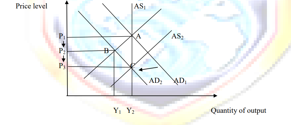
In short-run, the economy moves along the initial short-run aggregate supply curve AS1, going from point A to point B.
As the economy moves from point A to B, output falls from Y1 to Y2, and the price level falls
from P1 to P2.
The falling level of output indicates that the economy is in recession. Firms respond to lower sales and production by reducing employment. Thus pessimism about the future leads to falling incomes and rising unemployment.
What should policymakers do when faced with such recession?
They can take action to increase aggregate demand. An increase in government spending or increase in the money supply would increase the quantity of goods and services demanded at any price and therefore, shift the aggregate demand curve to the right. If policymakers can act with sufficient speed and precision, they can offset the initial shift in aggregate demand; return the aggregate demand curve back to AS1 and bring the economy back to point A.
Even without action by policymakers, the recession will remedy itself over period of time. Because of the reduction in aggregated demand, the price level falls. The fall in the expected price level alters wages, price level and perceptions; it shifts the short-run aggregate supply curve to the right from AS1 to AS2. This adjustment of expectants, allow the economy over time to approach point C, where the new aggregate demand curve (AD2) crosses the long-run aggregate supply curve.
In the new long-run equilibrium, point C, output is back to its natural rate. Even though the wave of pessimism has reduced aggregate demand, the price level has fallen sufficiently (to P3) to offset the shift in the aggregate demand curve. Thus in the long-run, the shift in the aggregate demand is reflected fully in the price level and not at all in the level of output.
NB/
In the short-run, shifts in aggregate demand cause fluctuation in the economy’s output of goods and services.
In the long-run, shifts in aggregate demand affect the overall price level but do not affect output.
7.2 THE EFFECTS OF A SHIFT IN AGGREGATE SUPPLY
Suppose that suddenly some firm experience an increase in their costs of production. For example, war in the Middle East might interrupt the shipping of crude oil, driving up the cost of producing oil products.
The macroeconomic impact of such an increase in production costs is that for any given price level, firms now want to supply a smaller quantity of goods and services. The figure below shows the short-run aggregate supply curve shifts to the left from AS1 to AS2
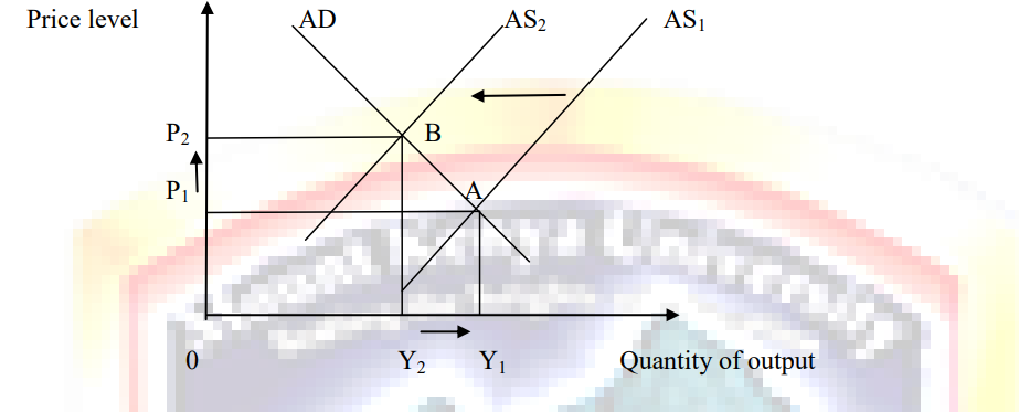
In the short-run, the economy moves along the existing aggregate demand curve, going from point A to point B. the output of the economy falls from Y1 toY2, and the price level rises from P1 to P2.
Because the economy is experience both stagnation (falling output) and inflation (rising prices) such an event is sometimes called stagflation.
What should policymakers do when faced with stagflation?
1. One possibility is to do nothing.
In this case, the output of goods and services remains depressed at Y2 for a while. Eventually, however, the recession will remedy itself as wages; prices and perception adjust to the higher production costs. A period of low output and high unemployment, for instance, puts downward pressure on worker’s wages. Lower wages, in turn, increase the quantity of output supplied. Overtime, as the short-run aggregate supply curve shifts backward AS1, the price level falls, and
the quantity of output approaches its natural rate. In long-run, the economy returns to point A, where the aggregate demand curve crosses the long-run aggregate supply curve.
2. Alternately, policymakers who control monetary and fiscal policy might attempt to offset some of the effects of the shift in the short-run aggregate supply curve by shifting the aggregate demand curve.
This possibility is as shown in the figure below.
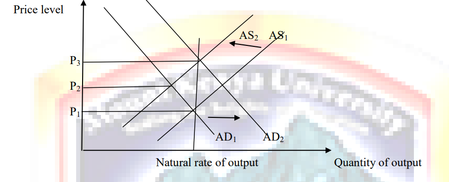
In this case, changes in policy shift the aggregate demand curve to the right from AD1 to AD2 i.e. exactly enough to prevent the shift in aggregate supply from affecting output. The economy moves directly from point A to point C. output remains at its natural rate, and the price level rises from P1 to p3. In this case, policymakers are said to accommodate the shift in aggregate supply because they allow the increase in costs to permanently affect the level of prices
NB
1. Shifts in aggregate supply can cause stagflation i.e. combination of recession (falling output) and inflation (rising prices)
2. Policymakers who can influences aggregate demand cannot offset both of these adverse effect simultaneously.
7.3 THE INFLUENCE OF MONETARY AND FISCAL POLICY ON AGGREGATE DEMAND
Imagine that you are a member of the Central Bank of Kenya Monetary Policy Committee (MPC), which sets Kenya monetary policy, you observe that the minister of finance has announced in his budget speech that he is going to cut government spending. How should the MPC respond to this change in fiscal policy?
To answer this question, you need to consider the impact of monetary and fiscal policy on the economy. Monetary and fiscal policies can each influence aggregate demand. Thus, a change in one of these policies can lead to short-run fluctuates in output and prices. Policymaker will want to anticipate this effect and, perhaps, adjust the other policy in response.
7.3.1 How monetary policy influences aggregate demand.
To understand how policies influence aggregate demand, one needs to examine the interest rate effect in more detail. The theory of liquidity preference shows how interest rate is determined. The theory is used to understand the downward slope of the aggregate demand curve and how monetary policy shifts this curve.
The theory of liquidity preference
John Maynard Keynes proposed the theory of liquidity preference to explain what factors determine the economy‟s interest rate. The theory is, in essence, just an application of supply and demand for money.
We have two type of interest rate, the nominal interest rate which is the interest rate as usually reported, and the real interest rate which is the interest rate corrected for the effects of inflation. For analysis purposes, expected rate of inflation is held constant. Thus, when the nominal interest rate rises or falls, the real interest rate that people expect to earn rise or falls as well. Development of theory of liquidity preferences by considers the supply and demand for money
and how each depends on the interest rate.
7.3.1.1 Money supply
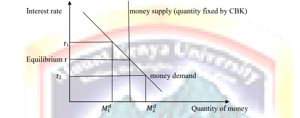
The first element of the theory of liquidity preference is the supply of money. The money supply is controlled by the central bank, such as central bank of Kenya. The central bank can alter the money supply by changing the quantity of reserves in the banking system through the purchase and sale of government bonds in outright open-market operations.
When the central bank buys government bonds, the money it pays for the bonds is typically deposited in banks, and this money is added to bank reserves. When the central bank sells government bonds, the money is received for the bond is withdrawn from the banking system and bank reserves fall. These changes in bank reserve, in turn, lead to
changes in banks‟ ability to make loans and create money.
In addition to these open-market operations, the central can alter the money supply by changing reserves requirements (the amount of reserves banks must hold against deposit) or the refinancing rate (the interest rate at which banks can borrow reserves from the central bank) If we assume that the central bank controls the money supply directly, then the quantity of money supplied in the economy is fixed at whatever level the central bank decides to set it.
Because the quantity of money supplied is fixed by central bank policy, it does not depend on other economic variables. In particular, it does not depend on the interest rate once the central bank has made its policy decision; the quantity of money supplied is the same, regardless of the prevailing interest rate. Fixed money supply is normally represented by a vertical supply curve as shown below.
7.3.1.2 Money demand
The second element of the theory of liquidly preference is the demand for money. As a starting point for understanding money demand, recall that any asset’s liquidly refers to the ease with which that asset is converted into the economy‟s medium of exchange.
Money is the economy’s medium of exchange, so it is by definition the most liquid asset available. The liquidly of the money explains the demand for it: people choose to hold money instead of other assets that offer higher rates of return because money can be used to buy goods and service.
Although many factors determine the quantity of money demanded, the one emphasized by the theory of liquidly preference is the interest rate. The reason is that the interest rate is the opportunity cost of holding money. That is, when you hold wealth as cash in your wallet, instead of as an interest-bearing bond, you lose the interest you could have earned. An increase in the interest rate raises the cost of holding money and, as a result, reduces the quantity of money demanded.
A decrease in the interest rate reduces the cost of holding money and raises the quantity demanded. Thus, as shown in the figure above money demand curve slope downward.
7.3.2 Equilibrium in the money market
According to the theory of liquidity preference the interest rate adjusts to balance the supply and demand for money. There is one interest rate, called equilibrium interest rate, at which the quantity of money demanded exactly balances the quantity of money supplied. If the interest rate is at any other level which is not equilibrium interest rate, people will try to adjust their portfolios of assets and as a result, drive the interest rate toward the equilibrium. For example, suppose that the interest rate is above the equilibrium level, such as r1 in figure above. In this case, the quantity of money that people want to hold, is less than the quantity of money that the central bank has supplied. Those people who are holding the surplus of money will try to get rid of it by buying interest bearing bonds or by depositing it in an interest-bearing bank account. Because bond issuers and bank prefer to pay lower interest rates, they respond to this surplus of money by lowering the interest rates they offer. As the interest falls, people become more willing to hold money until at the equilibrium interest rate, people are happy to hold exactly the amount of money the central bank has supplied.
Conversely, at interest rates below the equilibrium level, such as r2 in figure above. The quantity of money that people want to hold, is greater than the quantity of money that the central bank has supplied. As a result, people try to increase their holdings of money by reducing their holdings of bonds and other interest bearing assets.
As people cut back on their holdings of bonds, bond issuer find that they have to offer higher interest rates to attract buyers. Thus, interest rate rises and approaches the equilibrium level.
7.4 THE DOWNWARD SLOPE OF THE AGGREGATE DEMAND CURVE
The price level is one determinant of the quantity of money demanded. At higher prices, more money is exchanged every time a good or service is sold. As a result, people will choose to hold a larger quantity of money. That is, a higher price level increases the quantity of money demanded for any given interest rate. Thus, an increase in the price level from p1 to p2 shifts the money demand curve to the right from to as shown in panel (a) of figure below.
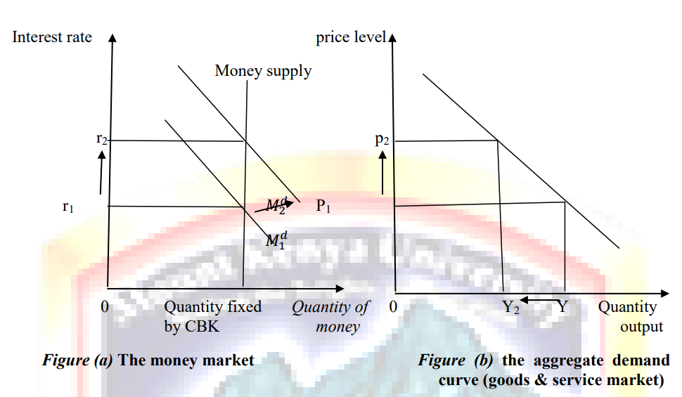
Shift in money demand affects the equilibrium in the money market. For a fixed money supply, the interest rate must rise to balance money supply and money demand. The higher price level has increased the amount of money people want to hold and has shifted the money demand curve to the right. Yet the quantity of money supplied is unchanged, so the interest rate must rise from r1 to r2 to discourage the additional demand.
This increase in the interest rate has ramification not any for the money market but also for the quantity of goods and services demanded, as shown in panel (b) of figure above. At higher interest rate, the cost of borrowing and the return to saving are greater. Fewer households choose to borrow to buy a new house, and these who do, buy smaller house, so the demand for residential investment falls. Thus, when the price level rises from P1 to P2, increasing money demand from MD1 to MD2 and raising the interest rate from R1 to R2, the quantity of goods and services demanded falls from Y1 to Y2.