
6.1 The model of aggregate supply and aggregate demand
The amount of output depends on the economy’s ability to supply goods and services, which in turn depends on the supplies of capital and labour and on the available production technology.
Flexible prices are crucial because prices adjust to ensure that the quantity of output demanded equals the quantity supplied. The economy works quite differently when prices are sticky. Output also depends on the demand for goods and services. Demand, in turn, is influenced by monetary policy, fiscal policy, and various other factors. Because monetary policy and fiscal policy can influence the country’s output over the time horizon, when price is sticky, price stickiness provides a rationale for why these policies may be useful in stabilizing the economy in the short run.
The model of aggregate supply (AS) and aggregate demand (AD) allows us to study how the aggregate price level and the quantity of aggregate output are determined. It also provides a way to contrast how economy behaves in ling-run and in short-run
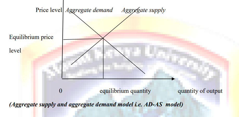
6.1.1 Aggregate demand (AD)
Aggregate demand is the total demand for final goods and services in the economy (Y) at a given time and price level. It is the amount of goods and services in the economy that will be purchased at all possible price levels.
Aggregate demand curve shows the relationship between the quantities of output demanded and the aggregate price level. In other words, the aggregate demand curve tells us the quantity of goods and services people want to buy at any given level of prices.
The figure below illustrates the aggregate demand curve as a downward sloping curve.
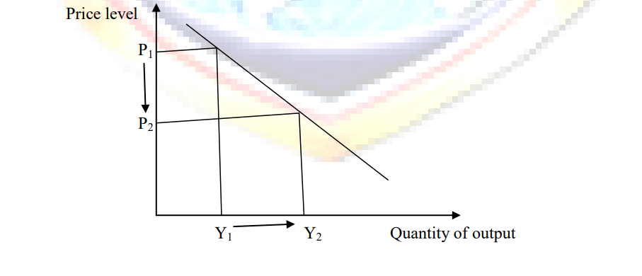
This means that ceteris paribus, a fall in the economy’s overall level of prices (from P1 to P2) tends to raise the quantity of goods and services demanded from (Y1 to Y2).
Why the aggregate demand curve slopes downward?
Why does a fall in the price level raise the quantity of goods and services demanded? To answer this question, recall that GDP (Y) is the sum of consumption (C), Investment (I), government purchases/spending (G), and net exports (NX).
Y=C+I+G+NX
Each of these four components contributes to the aggregate demanded for goods and services.
Assuming the government spending is fixed by policy, the other three components of spending (consumption, investment, and net exports) depends on economic conditions and, in particular, on the price level.
To understand the downward sloping of the aggregate demand curve, it is crucial to examine how the price level affects the quantity of goods and services demanded for consumption investments and net exports.
1. The price level and consumption (the wealth effect)
Consider the money that you hold in your wallet and your bank account. The nominal value of this money is fixed, but its real value is not. When prices fall, this money is more valuable because then it can be used to buy more goods and services. Thus, a decrease in the price level makes consumers wealthier, which in turn encourages them to spend more. The increase in consumer spending means a larger quantity of goods and services demanded.
2. The price level and investment (The interest rate effect)
The price level is one determinant of the quantity of money demanded. The lower the price level, the less money households need to hold to buy the goods and services they want. When the price level falls, households try to reduce their holdings of money by lending some of it out. For instance, a household might use its excess money to buy interest bearing bonds. Or it might deposit its excess money in an interest-bearing saving account, and the bank would use funds to
make more loans. In either case, as households try to convert some of their money into interestbearing assets, they drive down interest rates.
Lower interest rates, in turn, encourage borrowing by firms that want it invest in new factories and equipment and by households who want to invest in new housing. Thus, a lower price level reduces the interest rate, encourages greater spending on investment goods, and services demanded.
3. The price and net export (the exchange rate effect)
A lower price level lowers the interest rate. In response, some investors will seek higher returns by investing abroad. For instance, as the interest rate of Kenya government bonds falls, an investor might sell Kenya government bonds in order to buy other government bonds with better interest rate say US government bonds.
As investor tries to convert his shillings into dollars in order to buy the US bonds, he increases the supply of shillings in the market for foreign exchange. The increased supply of shilling causes the kenya shillings to depreciate relative to other currencies.
Because each shilling buys fewer units of foreign currencies, imports become more expensive to Kenyan residents. This change in real exchange rate ( the relative prices of domestic and foreign goods) increases Kenyan exports of goods and services and decreases Kenyan imports of goods and services.
Net exports, which equals export minus imports of goods and services increase. Thus, when a fall in the Kenyan price level causes its interest rates to fall, the real value of the shillings falls and this depreciation stimulates Kenyan net exports and thereby increases the quantity of goods and services demanded in the Kenyan economy.
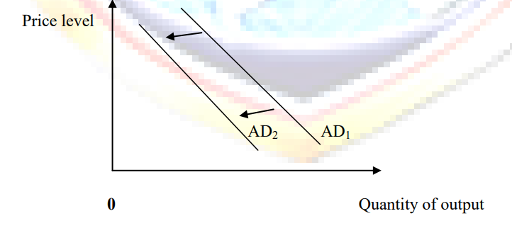
Why the aggregate demand curve might shift?
The demand slope of the aggregate demand curve shows that a fall in the price level raises the overall quantity of goods and services demanded. Many other factors, however, affect the quantity of goods and demanded at a given level. When one of these factors changes, the aggregate demanded curve shifts. The following are some example of events that shifts aggregate demand.
Shifts arising from consumption
Suppose people suddenly become more concerned about saving for retirement and, as a result, reduce their current consumption. Because the quantity of goods and services demanded at any price level is lower, the aggregate demand curve shifts to the left.
Conversely, imagine that a stock market boom makes people wealthier and less concerned about saving. The resulting increase in consumer spending means a greater quantity of goods and services demanded at any given price level, so the aggregate demand curve shifts to the right.
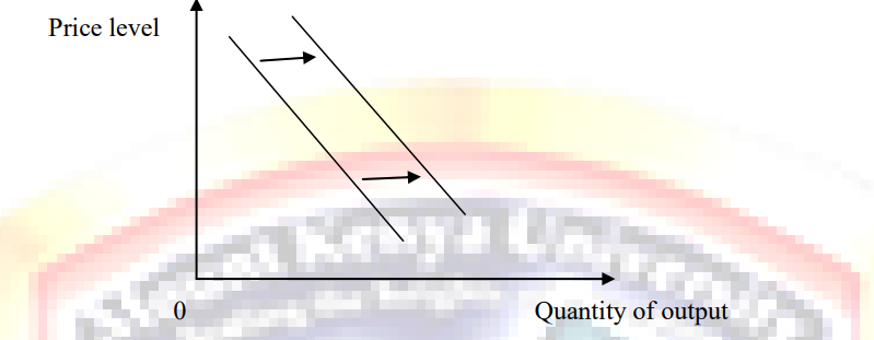
Thus, any event that changes how much people want to consume at a given price level shifts the aggregate demand curve.
One policy variable that has this effect is the level of taxation. When government cut taxes, it
encourages people to spend more.
Shifting arising from investment.
Any event that changes how much firms want to invest at a given price level also shifts the aggregate demand curve. If firms become pessimistic about future business conditions, they may cut back an investment spending, shifting the aggregate demand curve to left. Tax policy can also influence aggregate demand through investment. An investment tax credit (a tax rebate tied to a firm’s investment spending) increases the quantity of investment goods the firms demand at any given interest rate. It therefore shifts the aggregate demand curve to the right. The repeal of an investment tax credit reduces investment and shifts the aggregate demand curve to the left.
Another policy variable that can influence investment and aggregate demand is the money supply. An increase in money supply lowers the interest rates in the short-run. This makes borrowing less costly, which stimulates investment spending, and thereby shifts the aggregate demand curve to the right. Conversely, a decrease in the money supply raises the interest rate, discourages investment spending, and thereby shifts the aggregate demand curve to the left.
Shifts arising from government purchases/spending
The most direct way that policymaker shift the aggregate demand curve is through government purchases/spending. For example, suppose the government decides to reduce purchases of new weapons systems. Because the quantity of goods and services demanded at any price level is lower, the aggregate demand curve shifts to the left. Conversely, if the government starts building more motorways, the result is a greater quantity of goods and services demanded at any price level, so the aggregate demand curve shifts to the right.
Shift arising from net exports.
Any event that changes net exports for a given price level also shifts aggregate demand. For instance, when US experience a recession, it buys fewer goods from Kenya. This reduces Kenya net exports and shifts the aggregate demand for the Kenya economy to the left. Converse it true. Net exports sometimes change because of the movements in the exchange rate. Appreciation of local currency depresses net exports and shifts the aggregate demand curve to the left. Conversely depreciation of the local currency stimulates net exports and shifts the aggregate demand curve to the right.
6.1.2 Aggregate supply
Aggregate supply is the total supply of goods and services that forms in a national economy plan on selling during a specific time period. It is the total amount of goods and services that firms are willing to sell at a given price level in an economy.
The Aggregate supply curve
The aggregate supply curve tells us the total quantity of goods and services that firms produce and sell at any given price level. Unlike the aggregate demand curve, which is always downward sloping, the aggregate supply curve shows a relationship that depends crucially on the time being examined. In the long-run, the aggregate supply curve is vertical, whereas in the short-run the aggregate supply curve is upward sloping.
Why the aggregate supply curve is vertical in the long-run?
What determines the quantity of goods and services supplied in the long-run?
In the long-run, an economy’s production of goods and services (its real GDP) depends on its supplies of labour, capital and natural resources and on the available technology used to turn these factors of production into goods and services. Because the price level does not affect these long-run determinates of real GDP, the long-run aggregate supply curve is vertical as in the figure below
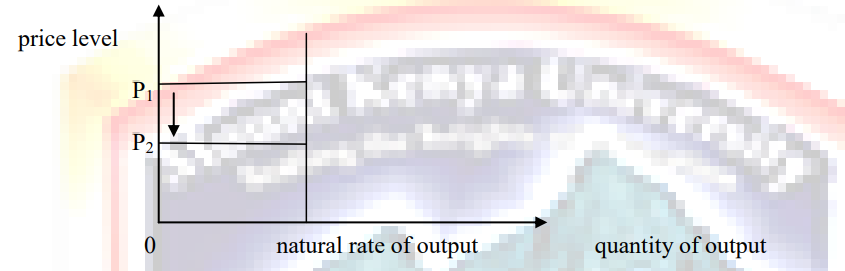
In other words, in the long-run, the economy’s labour, capital, natural resources and technology determine the total quantity of goods and services supplied, and this quantity supplied is same regardless of what the price level happens to be.
Why the long-run aggregate supply curve might shift?
The position of the long-run aggregate supply curve shows the quantity of goods and services predicted by classical macroeconomic theory. This level of production is sometimes called potential output or full-employment output. To be more accurate, we call it the natural rate output because it shows what the economy produces when unemployment is at its natural rate.
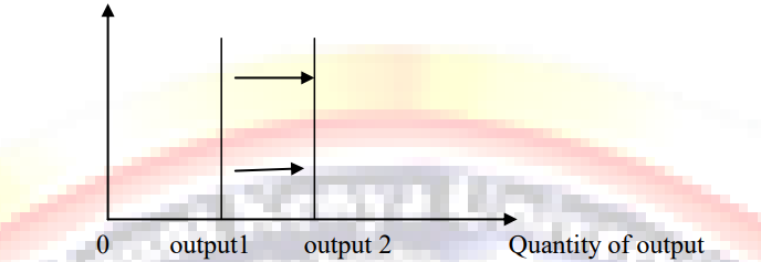
Any change in the economy that alters the natural rate of output shifts the long-run aggregate supply curve. Because output in the classical model depends on labour, capital, natural resources and technological knowledge, we can categorize shifts in the long-run supply curve as arising from these sources.
1. Shifts arising from labour.
The greater the number of workers the greater the quantity of goods and services supplied. As a result of an increase in number or workers, the aggregate supply curve would shift to the right. price level
If many workers left the economy to go abroad, the long-run aggregate supply curve would shift
to the left.
2. Shifts arising from capital.
An increase in the economy’s capital stock increases productivity and, thereby, the quantity of goods and services supplied. As a results, the aggregate supply curve shifts to the right. Conversely, a decrease in the economy’s stock decreases productivity and the quantity of goods and services supplied, shifting the long-run aggregate supply curve to the left.
3. Shifts arising from natural resources
An economy’s production depends on its natural resources, including its land, minerals and weather. A discovery of a new mineral deposit shifts the long-run aggregate supply curve to the right. A change in weather patterns that makes forming more difficult shifts the long-run aggregate supply curve to the left.
4. Shifts arising from technological knowledge.
Perhaps the most important reason that the economy today produces more than it did a generation ago is that our technological knowledge has advanced. The invention of the computer, for instance, has allowed as producing more goods and service from any given amount of labour, capital and natural resources. As a result, it has shifted to long-run aggregate supply curve to the right.
Conversely, if the government passed new regulation methods, perhaps because they are too dangerous for workers, the result would be a leftward shift in the long-run aggregate supply curve.
Why the aggregate supply curve slopes upward in the short-run.
In short-run, the aggregate supply curve is upward sloping as show in the figure below
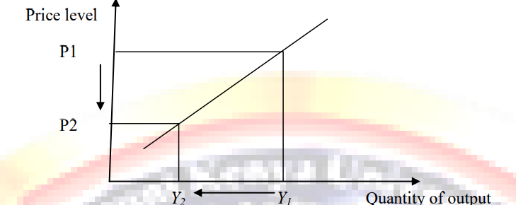
That is, over a period of a year or two, an increase in the overall level of prices in the economy tends to raise the quantity of goods and services supplied, and decrease in the level of prices tends to reduce the quantity of goods and services supplied.
Why might the short-run aggregate supply curve shifts
1. Shift arising from labour
An increase in the quantity of labour available (perhaps due to a fall in the natural rate of unemployment) shifts the aggregate supply curve to the right. A decrease in the quantity of labour available (perhaps due to a rise in the natural rule of unemployment) shifts the aggregate supply curve to the left.
2. Shifts arising from capital
An increase in physical or human capital shifts the aggregate supply curve to the right. A decrease in physical or human capital shifts the aggregate supply curve to the left.
3. Shifts arising from natural resources
An increase in the available of natural resources shifts the aggregate supply curve to the right.
4. Shifts arising from technology
Advance in technological knowledge shifts the aggregate supply curve to the right. A decrease in the available technology shifts the aggregate supply curve to the left.
5. Shifts arising from the expected price level
A decrease in the expected price level shifts the short-run aggregate supply curve to the right.
An increase in the expected price level shifts the short-run aggregate supply curve to the left.