
The Goods market also common known as the commodity or the product market is one where output (Y) is produced and later consumed by the economic agents. It is from the goods market that we have the national income identity, which we defined using the equation
Y = C + I + G
To develop this relationship we use a basic model called the Keynesian cross. In The General Theory Keynes proposed that an economy‘s total income was in the short run, determined largely by the desire to spend by households, firms and the government. The more people want to spend, the more goods and services firms can sell. The more firms can sell, the more output they will choose to produce and the more workers they will choose to hire.
Actual / Planned expenditures
Actual expenditure is the amount households, firms and the government spend on goods and services = GDP. Planned expenditure is the amount households, firms and the government would like to spend on goods and services. Actual differs from planned expenditure since firms engage in unplanned Inventory Investment because their sales do not meet their expectations.
For example
When firms sell less of their stock than they planned, their stock of inventories actually rise and vise verse. Since these unplanned changes in inventories are counted as investment spending by firms, actual expenditure can be either above or below planned expenditures. Now assuming closed economy planned expenditure is the sum of consumption, planned investment I, and government purchases G we can obtain the following equation.
E = C+I+G
C=C(Y-T) disposable Income
I=I
G=G
T=T
Substituting these equations in the planned expenditure equation we obtain
E = C(Y-T) + I + G
This equation shows planned expenditure as function of Y and the exogenous variables I, T and G. The relationship between planned expenditure and Income or Output can be graphed as shown below.
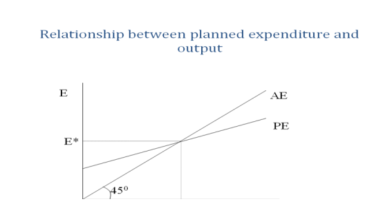
Planned expenditure depends on income because higher income leads to higher consumption, which is part of planned expenditure. The slope of the planned expenditure function is the marginal propensity to consume.
The Economy in Equilibrium
According to the Keynesian Cross the economy is in equilibrium when actual expenditure (AE) is equal planned expenditure (PE). This assumption is based on the idea that when people‘s plans have been realized, they have no reason to change what they are doing.
AE = PE
Y=E
This condition is held by plotting a 45-degree line as shown in the diagram above.
How does the economy get to the equilibrium?
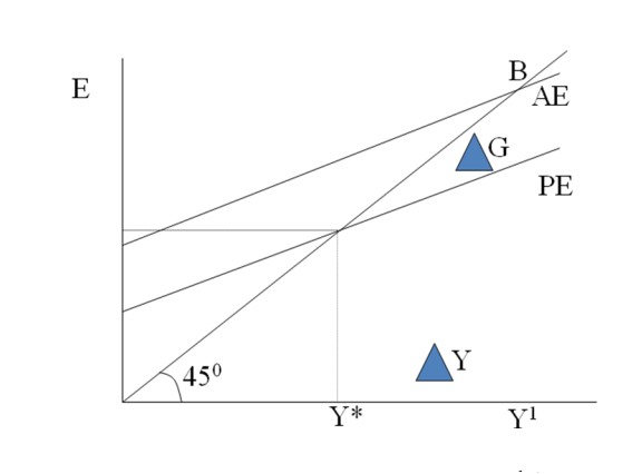
Inventories play an important role in the adjustment process Whenever the economy is not in equilibrium firms experience unplanned changes in inventories, and this induces them to change production levels. Changes in production in turn influences total income and expenditure moving the economy towards equilibrium.
• Equilibrium condition
For example whenever Y is below the equilibrium level, planned expenditure is greater than actual expenditure. Firms will meet the high levels of sales by drawing down their inventories.
To do so, they hire more workers and increases output.
• GDP rises and the economy approaches the equilibrium.
• On the other hand whenever Y is above the equilibrium level, planned expenditure is less than actual expenditure. Firms are selling less than they are producing.
• They add unsold goods to their stock of inventories.
• This unplanned rise in inventories induces firms to lay off workers and reduce production, and these actions in turn reduce GDP.
Effects of fiscal policy on planned expenditures
A fiscal policy is the policy of the government with regard to the level of government purchases, the level of transfers and the tax structure. Transfers are payments to households such as welfare to the poor and pensions to the elderly. They are the opposite of taxes. They increase households‘ disposable income, just as taxes reduce disposable income.
Govt. expenditures
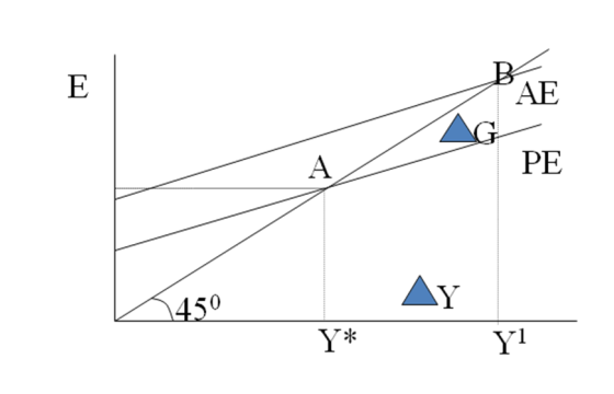
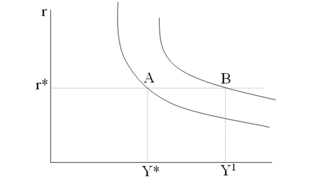
Consider how changes in government purchases affect the economy. Because government purchases are one component of expenditure, high government purchases result in high planned expenditure for any given level of income. If the government purchases rise by ΔG, then the planned-expenditure schedule shifts upwards by ΔG and the equilibrium moves from point A to
B.
An increase in government purchases
This graph shows that an increase in government purchases leads to an even greater increase in income. That is ΔY is larger than ΔG. The ratio ΔY/ ΔG is called the government multiplier. It tells how much income rises in response to a unit monetary value increase in government purchases. In this case it is greater than one.
Interest rate, investment and the IS curve
The Keynesian cross is basic to developing the IS-LM model. To be able to conclude our discussion, we introduce the investment function. The level of planned investment is a function of interest rate and is given as follows:
• I = I(r)
Is curve
The IS curve shows combinations of interest rates and levels of output such that planned spending equals income. (IS curve is a locus of all the points where the goods market is in equilibrium).It plots the relationship between the interest rate and the level of income that arises from the market for goods and services. To derive this curve, we use both The Keynesian cross and the Investment function.
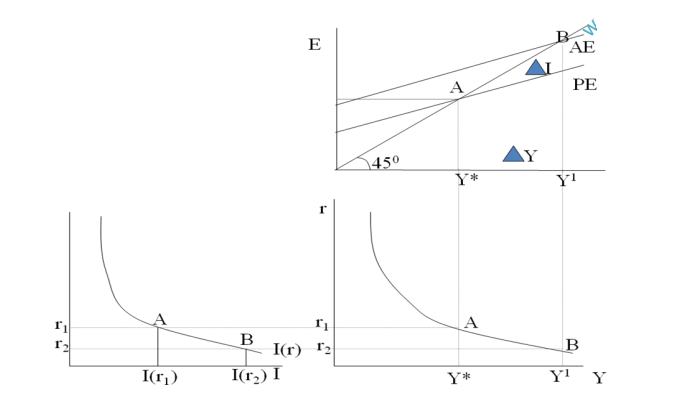
Panel A Shows the investment function, a decrease in the interest rate r1 to r2 increases planned investment. Panel B shows the Keynesian cross; an increase in planned investment shifts planed expenditure upwards and thereby increases income. Panel C shows the IS curve summarizing this relationship between interest rate and income. Higher interest rate lowers income. While lower interest rates rises national income. The IS curve is negatively sloped because an increase in the interest rate reduces planned investment spending and therefore reduce aggregate demand, thus reducing the equilibrium level of income.
Shifts in the IS Curve
As we learnt from the Keynesian Cross, the level of income depends on fiscal policy. The IS curve is drawn for a given fiscal policy: that is when we construct the IS Curve, we hold G and T fixed. When fiscal policy changes, the IS curve shifts. An increase in government purchases shifts IS curve outwards.
Panel A shows that an increase in government purchases raises planned expenditure. For any given interest rate the upward shift in planned expenditure leads to an income of Y of ΔG/(1- MPC).Therefore in panel B, the IS curve shifts to the right by this amount.
Loan able funds interpretation of the IS curve
Earlier we noted equivalence between the supply and demand for goods and the supply and demand for loan able funds. This equivalence provides a way to interpret the IS curve. Recall that the national income accounts identity can be written as
Y-C-G = I
S = I
The left hand side of this equation is national savings S, and the right-hand side is Investment, I. National savings represent the supply of loanable funds and investment represents the demand for these funds. Assuming
C = C(Y-T)
We obtain
Y –C(Y-T)-G = I(r)
The left hand side shows that the supply of loanable funds depends on income and fiscal policy. The right hand side shows that demand for loanable funds depends on the interest rate. The interest rate adjusts to equilibrate the supply and demand for loans.
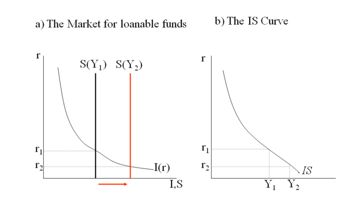
Panel A shows that an increase in income from Y1 to Y2 raises savings and thus lowers equilibrium interest rates interest rates. Panel B expresses this negative relationship between interest rates and income. In this regard the IS curve can be interpreted as showing the interest that equilibrates the market for loanable funds given any level of income. With an increase in income, national savings increase, hence an increase in the supply for loanable funds. This leads to a fall in interest rates and the IS curve summarizes this relationship. Thus higher incomes lead to low levels of interest rates. For this reason the IS curve is downward sloping.
4.2 Money Market
4.2.1 Define the LM curve
The LM curve plots the relationship between interest rate and the level of income that arises in the market for money balances. To understand this relationship, we begin by looking at a theory of the interest rate; called the theory of liquidity preference. In his book ―General Theory‖, Keynes offered his view of how the interest rate is determined in the short run. He argued that interest rate adjusts to balance the supply and demand for the economy‘s most liquid asset money.
Supply for real money balances
If M stands for the supply of money and P stands for the price level, Then M/P is the supply of real money balances. The theory of liquidity preferences assumes there is a fixed supply of real money balances. The money supply M is an exogenous policy variable chosen by a central bank. The price level P is also an exogenous variable in this model. These assumptions imply that the supply of real balances is fixed, in particular does not depend on interest rate.
Demand for real money balances
The theory of liquid preference posits that interest rate is one of the determinants of how much money people choose to hold. The reason is that the interest rate is the opportunity cost of holding money; it is what you forgo by holding some of your assets as money, which does not bear interest, instead of as interest bearing bank deposits or bonds. When interest rates increase people want to hold less of their wealth in the form of money balances. Thus, we can write the demand for real money balances as The dd curve slopes downwards because higher interests rates reduce the quantity of the real balances demanded. This theory argues that the interest rate adjusts to equilibrate the money market. At the equilibrium interest rate, the quantity of real balances demanded equals the quantity supplied
• How does adjustments for equilibrium happen
• The adjustment occurs because whenever the money market is not in equilibrium, people try to adjust their portfolios of assets and , in the process, alter the interest rate –
• e.g. if interest rate is above the equilibrium level, the quantity of real balances supplied excess the quantity dd. Individuals holding the excess supply of money try to convert some of their non-interest –bearing money into interest – bearing bank deposits or bonds.
• Banks and bond issuers, who prefer to pay lower interest rates, respond to this excess
supply of money by lowering the interest rate they offer.
• Conversely if interest rate is below equilibrium level so that quantity of money demanded exceeds the quantity of money supplied, individuals try to obtain more money by selling bonds on making bank withdrawals. To attract now scarcer funds, bank and bond issuers respond by increasing the interest rate they offer.
Derivation of the LM curve
Before we derive the LM curve it is important to consider how a change in economy‘s level demand for money. When income is high, expenditure is high, so people engage in more of income affects the market for real money balances. The level of income affects the transactions that require the use of money. Thus, greater income implies greater money demand. This can be expresses using the money demand function as follows:
The quantity of real money balances demanded is negatively related to the interest rate and positively related to income. Using the theory of liquidity preference we can figure out what happens to equilibrium interest rate when the level of income changes. A change in the level of income, given fixed supply of real money balances leads to a rise in interest rates. Therefore according to the theory of liquidity preference, higher income leads to a higher interest rate.
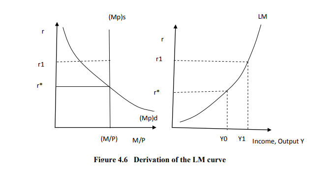
The LM curve plots this relationship between the level of income and interest rate. The higher the level of income, the higher the demand for real money balances, and the higher the equilibrium interest rate. For this reason, the LM curve slopes upward.
Shifts in the LM curve
The LM curve tells us the interest rate that equilibrates the money market given any level of income. Interest rate too depends on the supply of real balance, M/P. This means that the LM curve is drawn for a given supply of real money balances. If real balances change- for- example, if the central bank alters the money supply- the LM curve shifts.
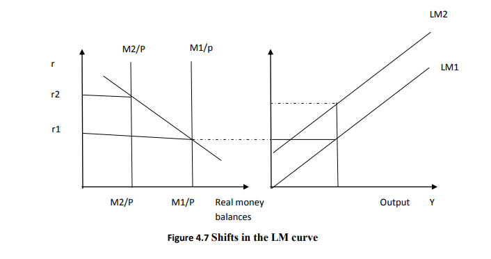
In summary, the LM curve shows the combinations of the interest rate and the level of income that are consistent in the market for real money balances. The LM curve is drawn for a given supply of real money balances. Decreases in the supply of real money balances shift the LM curve upwards. An increase in the supply of real money balances shifts the LM curve downwards.
A Quantity-Equation Interpretation of the LM Curve
Money x Velocity = Price x Income
M x V = P x Y
P is the price of a typical transaction- the number of monetary value exchanged. M is the quantity of money. V is called the transactions velocity of money and measures the rate at which money circulates in the economy. In other words, velocity tells us the number of times a monetary value bill changes hands in a given period of time. Assuming that velocity is constant, it implies that for any given price level (P) the supply of money by itself determines the level of income Y. Since Y does not depend on interest rate the quantity theory is equivalent to a vertical LM curve.
How do we realize the more realistic upward sloping LM curve ?
By relaxing the assumption of constant velocity of money. The assumption that V is constant derives from the assumption that the demand for real money balances depends on income. Yet we have so far seen that the demand for real money balances also depends on interest rates. Higher interest rates rises the costs of holding money and reduces money demand. Hence the velocity of money must increase when people respond to higher interest rate by holding less money: Each coin they hold must be used more often to support a given volume of transactions. We can write this as
MV(r) = PY
The velocity function V(r) indicates that velocity is positively related to the interest rate. This form of the quantity equation yields an LM curve that slopes upwards. Because an increase in the interest raises the velocity of money, it raises the level of income for
any given money supply and price. The LM curve expresses this positive relationship between the interest rate and income.
• This equation shows why changes in money supply shift the LM curve. For any given interest rate and price level, the money supply and the level of income must move together.
• NB: Quantity equation is only is just another way to express the theory behind the LM curve.
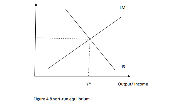
Short-Run Equilibrium
The short run equilibrium is represented by the ISLM model. Whereas the IS curve represents equilibrium in the goods market the LM curve represents equilibrium in the money market. The Lm curve by itself does not determine either income or interest rates that will prevail in the economy. Just like the IS curve, the Lm curve is only a relationship between these two endogenous variables. The Lm and the IS curve together determine the economy’s equilibrium. The intersection of the two curves determines output and interest rates in the short run, that is, for a given price level. Expansionary fiscal policy moves the IS curve to the right, raising both income and interest rates. Contractionary fiscal policy moves the IS curve to the left, lowering both income and interest rates.
Explaining fluctuations in the economy with the ISLM curve
The intersection of IS and LM curves determines the level of incomes. When one of the curves shifts short run equilibrium of the economy changes and National Income fluctuates.‘ A change in fiscal policy for instance will shift the IS curve e.g fiscal expansion shifts the IS curve to the right. Consider an increase in government purchases at unchanged interest rates, higher levels of government spending increase the level of aggregate demand .To meet the increased demand for goods, output must increase Expansionary monetary policy moves the LM curve to the right, raising income and lowering interest rates.
• Contractionary monetary policy moves the LM curve to the left lowering the level of income and raising the interest rates.
4.3 Crowding Out and Liquidity Trap
Crowding out occurs when expansionary fiscal policy causes interest rates to rise, thereby reducing private spending, particularly investment. As interest rate increases due to increased government spending, crowding out effect is greater. Liquidity trap is a situation whereby prevailing interest rate are low and saving rates are high making the monetary policy ineffective.. People choose to void bonds and prefer to keep their funds in savings because they believe that interest rates will soon rise. In a liquidity situation the
demand fro money is imperfectly inelastic i.e it is horizontal. This means that further injections of money in the economy will not serve to further lower the interest rate
If the economy is in liquidity trap, and thus the LM curve is horizontal, an increase in government spending has its full multiplier effect on the equilibrium level of income. There is no change in interest rates associated with the change in government spending, and thus no investment spending is cut off. If the LM curve is vertical, an increase in government spending has no effect on the equilibrium level of income and increases only the interest rate. If the government spending is higher and output is unchanged, there must be an offsetting reduction in private spending. In this case, the increase in interest rates crowds out an amount of private spending particularly investment equal to the increase in government spending. Thus there is full crowding out if the LM curve is
vertical.
Importance of Crowding Out
Assuming that prices are given and that output is below the full-employment level. When fiscal expansion increases demand, firms can increase output level by hiring more workers. In real life crowding out occurs through a different mechanism as high demand leads to high price levels and a reduction in real money balances. Also, in an economy that is not fully utilizing its recourses, there can never be full crowding out since the LM curve is not vertical. Crowding out is therefore a matter of degree. Thirdly, with unemployment, and low output levels, interest rates need not rise at all when government spending rises, and there need not be any crowding out. This is true because the monetary authorities can accommodate the fiscal expansion by an increase in the money supply.
The Transmission Mechanism of a monetary policy
The processes by which changes in monetary policy affect aggregate demand are essential. The first is that an increase in real money balances generates portfolio disequilibrium; that is, at the prevailing interest rate and level of income, people are holding more money than they want. As a result they start depositing extra money in banks or use it to buy bonds. The interest rate r then falls until people are willing to hold all the extra money created and this brings the money market to equilibrium. The lower interest rates stimulate planned investment, which increases planned expenditure, production and income. This process is commonly known as the monetary
transmission mechanism.