8.0 Introduction
The IS-LM model is an aggregate demand model which gives best interpretation of Keynesian short-run macroeconomic model. The model takes price level as exogenous variable and shows what determines national income.
IS-curve defines equilibrium in the goods market. IS stands for investment and saving, therefore
IS-curve represents what’s going on in the market for goods and services.
LM-curve describes equilibrium in the money market. LM stands for liquidity and money and therefore, LM curve represents what‟s happening to the supply and demand for money. Because the interest rate influences both investments and money demand, interest is the variable that links the two halves of the IS-LM model. The IS-LM model shows how interactions between these markets determine the position the position and slope of the aggregate demand curve and, therefore, the level of national income in the short run.
8.1 The IS-curve
An IS-curve shows combinations of interest rate and income/output that equilibrates the goods market. The curve slopes downwards from left to right. Change in government spending, taxation and investment shifts the IS-curve.
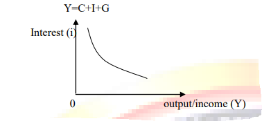
The IS-curve is derived from the Keynesian cross. Keynes, in his general theory, proposed that an economy’s total income was, in the short run, determined largely by the desire to spend by households, firms and government. The more goods and services firm can sell. The more firm can sell, the more output they will choose to produce and the more workers they will choose to hire. Thus, the problem during recessions and depressions, according to Keynes, is as a result of inadequate spending. The Keynesian cross is the attempt to model this insight.
The slope of IS-curve depends on:
1. Responsiveness of investment spending to changes in interest rate. This is represented by the size of investment coefficient. If this coefficient is large, investment spending is sensitive to interest rate i.e. the IS-curve will be relatively flat. If the coefficient is
small, IS-curve will be relatively steep.
2. The spending multiplier – a higher multiplier means a flatter is curve and low multiplier implies steeper IS-curve.
Thus a large investment coefficient and small multiplier gives a flatter IS-curve while a small investment coefficient and high spending multiplier gives a steeper IS-curve.
Factors that shifts the IS-curve
- Changes in autonomous consumption
- Changes in government spending
- Changes in taxation
- Changes in investment
- Changes in net exports ( for open economy)
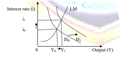
An expansionary fiscal policy involves either increase in government spending or a tax cut. This shifts the IS-curve out to the right. Thus increasing both level of output and interest rate.
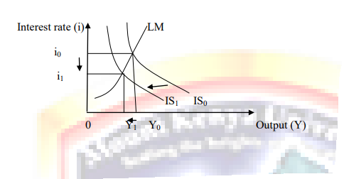
Conversely, a contractionary fiscal policy involves either reduction in government spending or increase in taxes. This shifts the IS-curve inward to the left, thus reducing both output and interest rate
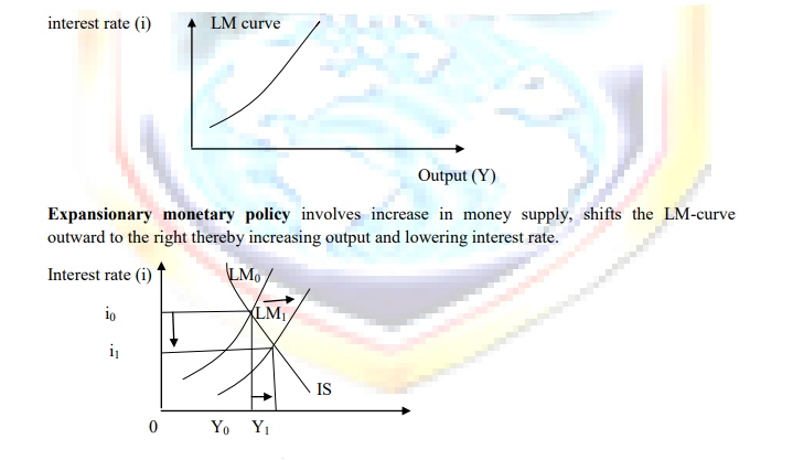
8.2 The LM-curve
The LM-curve describes equilibrium in the money market. LM-curve shows combination of
interest rate (i) and output (Y) that equilibrates money market for a given level of income. LMcurve slopes upwards from left to right
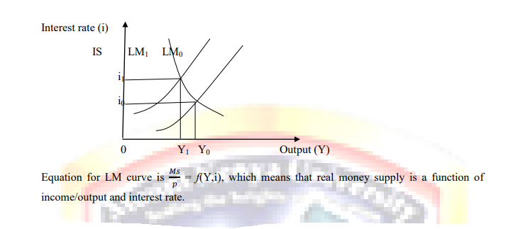
Contractionary monetary policy involves a reduction in money supply. This shifts LM-curve up to the left causing a reduction in output and an increase in interest rate.
Factors that shift LM-curve:
- Factors that affect real money supply such as change in money supply and changes in prices.
- Factors affecting money demand such a changes in income and changes in interest rate.
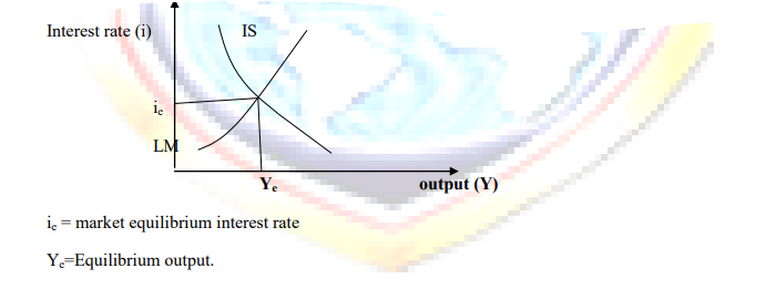
8.3. General equilibrium
General equilibrium in the economy is obtained when the IS-curve intersects LM-curve i.e. when goods and services markets and money markets are in equilibrium. The IS-LM model is a short run analytical model.
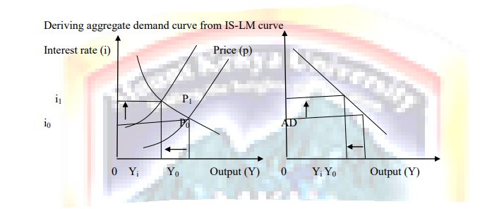
8.4 IS-LM model and aggregate demand
IS-LM model is a short run model where prices are assumed fixed. In the long run, prices do change. When prices change, the LM curve shifts, thereby affecting the level of income in the economy. The aggregate demand function describes the relationship between price level (P) outputs (Y).
To determine the aggregate demand function we examine what happens to the IS-LM model when price level changes. We derive the aggregate demand curve by assuming price increases from P0 to P1 holding Money supply constant. An increase in price level shifts LM-curve up to the left reducing output and raising interest rate.