5.1 Mundell- Fleming Model
This is an open – economy version of the IS- Lm model. Both the Mundell- Fleming Model And IS-LM model assume that the price level is fixed and then show what cause short – run fluctuation in aggregate income. The key difference is that the IS- LM model assumes a closed economy, whereas the Mundell- Fleming model assumes an open economy.
The Key Assumptions of the model
- The model assumes that the economy being studied is a small open economy with perfect capital mobility. That is, the economy can borrow or lend as much as it wants in the world financial market and, as a result, the economy‗s interest rate is determined by the world interest rate. Mathematically we can write this assumption as r= r*
- The world interest rate is assumed to be exogenously fixed because the economy is sufficiently small relative to the world economy that it can borrow or led as much as it wants in world financial markets without affecting the world interest rate. Perfect capital mobility implies that if some events were to occur that would normally raise the interest rate such as a decline in domestic saving in a small open economy , the domestic interest rate might rise by a little bit for a short time, but as soon as it did , foreigners would see the higher interest rate and start lending to this country by instance buying the country‘s bonds. The capital inflow would drive the interest rate back toward r*. Similarly if there were any event that were to start driving the
domestic interest rate downwards, capital would flow out of the country to earn a higher abroad , and capital outflow, would drive the domestic interest rate back toward , the r= r* equation represents the assumption that the international flow of capital is sufficiently rapid as to keep the domestic interest rate equal to the world interest rate. - The model also assumes that price levels at home and abroad are fixed , this means that the real exchange rate appreciate , foreign goods become cheaper compared to domestic goods and this cause export to fall and import to rise.
5.2 The Goods Market and the IS Curve
The Mundell- Fleming model is describes the market for goods and services much as the IS- LM model does, but it adds a new term for net export. In particular, the goods market is represented with the following equation.
Y= C(Y-T) +Ir* + G+NX (e)
This equation states that aggregate income is the sum of consumption C, investment I, government purchase G, and net export NX.
- Consumption depends positively on disposable income-T.
- Investment depends negatively on the interest rate, which equals world interest rate r*.
- Net exports depend negatively on the nominal exchange rate e. As before, we define the exchange rate the amount of foreign currency per unit of domestic currency. For example, e might be Kshs 75 per dollar.
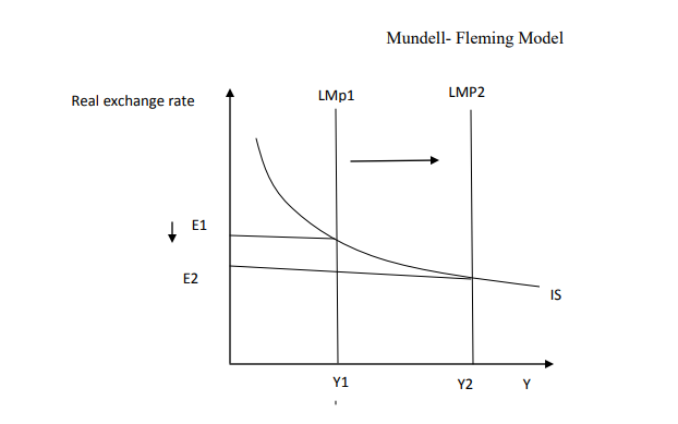
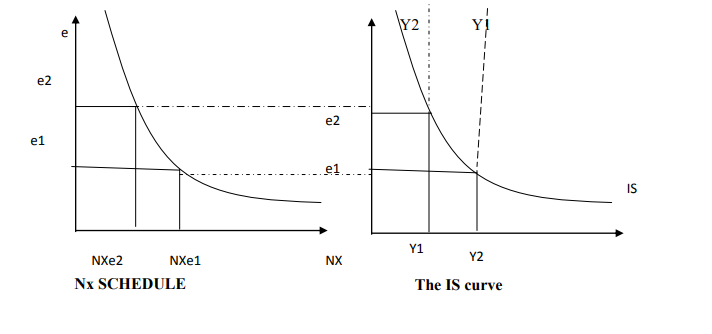
From the diagram below, the IS curve slopes downward higher interest rate reduce net export which in turn reduce the aggregate income. Using the diagram below a change in the exchange rate from e1 to e2 lowers net from NX (e) to NX (e2). In panel b the reduction falls from Y2 to Y2. The IS curve summarizes this relationship between the exchange rate and the level of income Y in panels c.

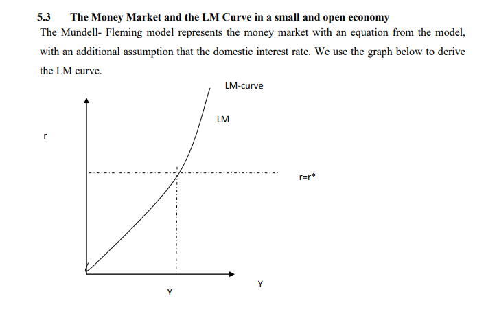
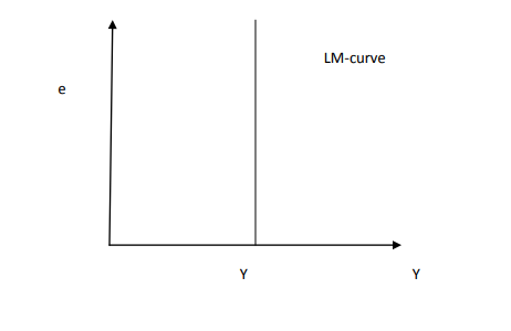
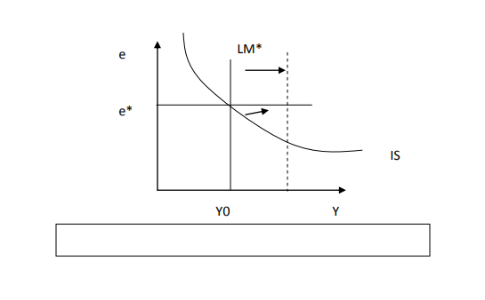
The figure above shows the standard way of representing the LM curve, together with a horizontal line representing the world interest rate r* . The intersection of the two curves determines the level of income regardless of the exchange rate. Therefore the LM curve is
vertical.
A small Economy Short Run Equilibrium
According to the model – fleming model, a small open with perfect capital mobility can be described by two equation:
Y= C(Y-I) +I(r*) + -G-NX(e)………………………………………….IS
MP=L(r*,Y)…………………………………………………………………..LM
The first equation describe the goods market ,and the second equation describe the money market . The exogenous valuable are fiscal policy G and T , monetary policies M, the price level P and the world interest rate r* . The endogenous variable are income Y and the exchange rate. These two relationship are illustrated together in the figure below.
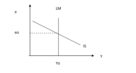 The intersection of the IS curve and the LM curve shows the exchange rate and the level of income at which both the goods market and the money market are in equilibrium.
5.4 Effects of Fiscal Policies in A Small and Open Economy
Before analyzing the impacts of policies in an open economy, it is important to specify the interaction monetary system in which the country has chosen to operate. There are three systems that a country operates:
- Floating exchange rates
- Fixed exchange rate
- Flexible exchange rates
The most common is the floating exchange rate, where the exchange rate is allowed to fluctuate freely in response to changing economic conditions.
Effects of fiscal policy on the Floating Exchange Rates.
Consider an increase as in government purchase or a tax cut. An expansionary fiscal policy increased planned expenditure, & shift the IS curve to the right. As a result, the exchange rate appreciates, while the level of income remains the same.
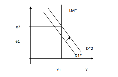
This yields very difference results from those of closed economy. As soon as the interest rate to increase above world interest rate, capital flows in from abroad. This capital inflow increase the demand for domestic currency in the market for foreign currency exchange and , thus bids up the value of the domestic currency . The appreciation of the exchange rate makes domestic goods expensive relative to foreign goods, and this reduces net export. The fall in net export offsets the effects of the expansionary fiscal policy on income.
The reasons why the fall in net export is so great to render fiscal policy completely powerless to influence income has to do with the money market . At the world interest rate, there is only one level of income that can satisfy the level of real money balance due this level of income does not change when fiscal policy change . Thus when an expansion fiscal policy is pursued , the appreciation of the exchange rate and the fall in net export must be exactly large enough to offset fully the normal expansionary effects of the policy on income
Effects of Monetary policy on floating exchange rates
Now let‘s consider an increase in money supply by central bank. Because the price level is assumed to BE fixed, the increase in the money supply means an increase in real balances. The increase in balances shifts the LM curve to the right.
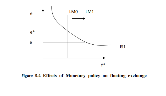 Although monetary policy influence income in an open economy , as it does in a closed economy , the monetary transmission mechanism is different from a small open economy , because the interest rate is fixed by the world interest rate. As soon as an increase in money supply puts downwards pressure on the domestic interest rate , capital flows out of the economy as investors seek a higher return elsewhere. This capital outflow prevents the domestic interest rate from falling. In addition , because the capital outflow increases the supply of the domestic currency in the market for foreign – currency exchange rate makes domestic goods inexpensive relative goods and thereby , stimulate net export . Hence, in a small open economy, monetary policy influences income by altering the exchange rate rather than the interest rate.
Effect of Trade Policy on floating exchange rates
Suppose that the government reduces the demand for imported goods by imposing an import quota or a tariff. Because net export equals export minus import, a reduction in imports means an increase in net that is , the net export schedule shift to the right . This shift in the net export schedule increases planned expenditure and thus moves the IS curve to the right . Because the LM curve is vertical, the trade restriction raises the exchange rare but does not income. Often a stated goal of policies to restrict trade to alter the trade balances NX. Such policies do not necessarily have that effect. The same conclusion holds in the Mundell- Fleming model under floating exchange rates. Recall that.
Nx(e) =Y-C\(Y-T) –I(r*)-G
Because a trade restriction does not effects income , consumption , investment or government‘s purchases , it does not affects the trade balance. Although the shift in the net export schedule tends to raise NX , the increase in the exchange rate reduces NX by the same amount.
5.5 The Small Open Economy under Fixed Exchange Rates
We now turn to the second type of exchange rate – system fixed exchange rates. This system was in operation in the 1950s and 1960s and was later by floating exchange rate system .Later in the 1970s some European countries reinstated this system and some economic have advocated a return to a worldwide system of fixed exchange rates. In this section we discuss how this system works, and we examine the impact of economic policies on an economy with a fixed exchange rate.
A Fixed exchange Rate System
Under a fixed system of fixed exchange rates, a central bank stands ready to buy or sell the domestic currency for foreign currencies at a predetermined price. Suppose, for example hat the central bank of Kenya announced that it was going to fix the exchange rate at Ksh 20 per dollar. It would then stand ready to give kshs20 shilling in exchange for a dollar or give out dollar in exchange for Kshs.20 .to carry out policy , the Central Bank of Kenya would need a reserve of Kenya shilling ( which it can print) and a reserve of dollars ( which it must have purchased previously)
A fixed exchange rate dedicates a country‘s monetary policy to the single goals of keeping the exchange rate at the announced level. In other words , the essence of a fixed – exchange rate system is he commitment of central bank to allow the money supply to adjust to whatever level will ensure that the equilibrium exchange rate equals the announced rate . Therefore so long as the central bank is ready to buy a sell foreign currency at the fixed exchange rate, the money supply adjusts automatically to the necessary level.
Fiscal Policy and Fixed exchange Rate System Let‘s now examine how a fiscal policy affects a small open economy with a fixed exchange rate. Consider an increase in government spending. This policy shifts the IS curve to the right as in the figure below.
This puts an upwards pressure on the exchange rate. But because the central bank stands ready to trade foreign and domestic currency at the fixed exchange rate, arbitrageurs quickly respond to the rising exchange rate by selling foreign currency to the central bank , leading to an automatic monetary expansion . The rise in money supply shifts the LM curve to the right and raise aggregate income.
Monetary Policy and fixed exchange Rate System
Consider an increase in money supply by the central bank for example by buying bonds from the public. The initial impacts of this policy to shift the LM curve to the lowering the exchange rate.
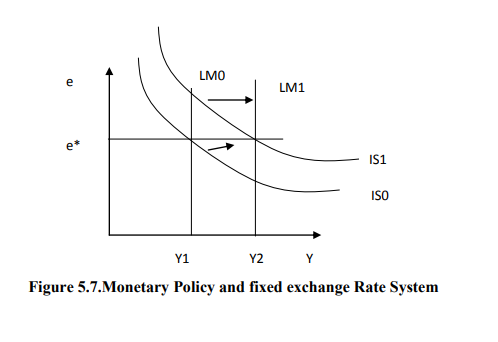
But because the central bank is committed to trading foreign and domestic currency at a fixed exchange rate, arbitrageurs quickly respond to the falling exchange rate by selling the domestic currency to the central bank , causing the money supple and LM curve to return to their initial position. Hence monetary policy is ineffective under a fixed exchange rate. By agreeing to fix the exchange rate, the central bank gives up control over the money supply.
A country with a fixed exchange rate , can , however , conduct a type of monetary policy ; it can decide to change the level at which the exchange rate is fixed . A reduction in the value of the currency is called devaluation; an increase in the value of the currency is called a revaluation
Trade policy and fixed exchange Rate System
Suppose the government reduces imports by imposing an import quota or a tariff. This policy shifts the net export schedule to the right and this shifts the IS curve to the right as in the figure below.
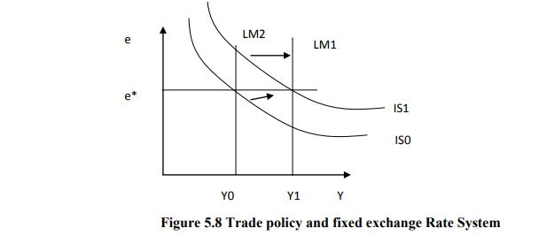
The shift in the IS curve tends to raise the exchange rate. To keep the exchange rate at the fixed level, the money supply must rise, shifting the LM curve to the right. Thus a trade restriction under a fixed exchange rate system induces monetary expansion rather than an operation in the exchange rate. The monetary expansion in turn increases aggregate income. When income rises, saving also rises, and this improves an increase in net exports.
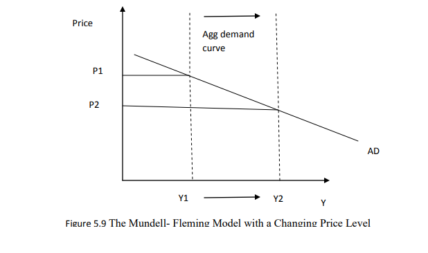
5.6 The Mundell- Fleming Model with a Changing Price Level
So far we have been using the Mundell – Fleming model with study the small open economy in the short run when the price level is fixed. To examine price adjustment in an open economy, we must distinguish between the nominal exchange rate e , which equals ep/p* . We can then write the Mundell- Fleming model as
Y= C(Y-T) I(r*) +G+NX (E)……………………………….IS
M/P= L(r*, Y)……………………………………………….LM
The figure below shows what happens when the price level falls. Because a lower level raise the level of money balances, the LM shifts to the right. The exchange rate depreciate and the equilibrium level of income rises. The aggregate demand curve summarizes this income shifts the aggregate demand curve to the right . Policies that lower income shift the aggregate demand curve to the left.