

Purpose The theory of demand and supply enables us to understand the determination of prices and quantities in different markets. For example, why the prices of agricultural commodities such as tomatoes, apples, mangoes and cabbages increase and decrease at certain times of the year, why have the prices of computers, music systems and television sets been steadily declining over time. An understanding of the working of the price system provides us with the answers to some of these questions. The price system provides the basis for determining the prices of factors of production.
Specific Objectives
At the end of this lesson you should be able to:
- Outline the key determinants of demand and supply
- Explain the difference between a movement along a demand and supply curve and shift of the curve.
- Explain the concept of market equilibrium
- Distinguish between maximum and minimum price controls and explain the consequences of each
- Compute equilibrium values in elementary market models.
2.1 Definition of Demand
Demand refers to the quantity of a commodity that consumers are willing and able to purchase at any given price over a given period of time. It is important to realize that demand is not the same thing as want, need or desire. Only when want is supported by the ability and willingness to pay the price does it become an effective demand and have an influence on the market price. Hence demand in economics means effective demand. It is different from desire in that it has to be supported by the ability to purchase the product/service. The price of a commodity is most important factor/determinant of demand. All factors affecting demand other than the price are referred to as conditions for demand. While analyzing the relationship between price and quantity of demand economists assume that all factors affecting demand remain constant. An individual demand for a given good can be presented in a form of a demand schedule. A demand schedule is a table showing quantity of a commodity that could be purchased at various prices. The Table 2.1 shows an individuals demand for commodity X
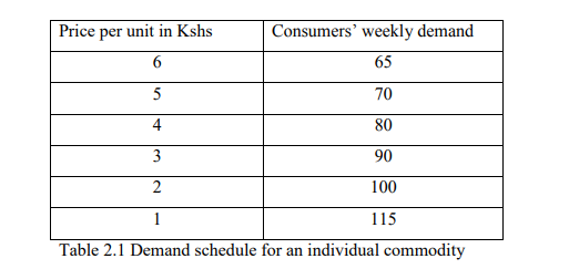
From the table, 65 units of commodity X will be demanded per week if the price is Kshs 6 per unit. A demand schedule can be represented in the form of a graph known as a demand curve. Figure 2.1 shows the demand curve for commodity X. The curve shows graphically the relationship between quantity demanded and the price of the commodity. A demand curve has a negative slope. It slopes downwards from left to right showing that as the price of a commodity falls demand increases. The inverse relationship between the price of a commodity and the quantity demanded is what is referred as the law of demand.
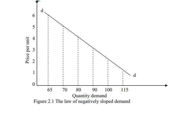
This law states that, “ceteris paribus (other things remaining constant), the lower the price of a commodity the greater the quantity demanded by the individual and vice versa”.
Exceptions to the Law of Demand
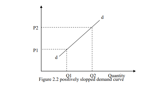
There are some demand curves that slopes upwards from left to right showing that as the prices of a product rise more is demanded and vice versa. This type of demand curve is known as regressive, exceptional or abnormal demand curve and occurs in the following
situations:
- When there is fear of a more drastic price changes in the future. This will causes consumers to increase there quantity demanded to avoid paying a higher price in the future. This situation is often found in the stock exchange where there is often an increase in the demand of shares of a company if its shares are expected to increase.
- In the case of giffen goods. This refers to basic foodstuffs that constitute a high proportion of the budget of low income families. When the price of a giffen good rises, the proportion of the total income of individuals who consumes these giffen goods rises and since such consumers are worse off in real terms, they can no longer afford to consume other more expensive commodities like meat and fruits. To make up for the goods they can no longer afford to buy, they are more likely to purchase more of basic
foodstuffs; conversely when the price of basic foodstuffs falls. They become better of in real terms and are likely to buy more or relatively more expensive foodstuffs and less basic foodstuffs.
Goods of ostentation (Veblen goods). These are commodities whose prices falls in the upper price ranges and that have a snob appeal. The wealthy are usually concerned about status. Believing that only goods at high prices are worth buying and worth the effect of distinguishing them from other consumers. In the case of such commodities, a firm increasing its prices may find that the sales of its product increase and at lower prices less of the commodity may be bought as the commodity is rejected as being substandard.
Consumers often in making comparisons between similar products with different prices opt for relatively more expensive product believing it to be better. As prices increase demand increases this is referred to as sonob effect. Examples of goods of ostentation are expensive perfume, jewellery, cars clothes, etc. The demand curve will be positively slopping as indicated in Figure 2.2.
2.2 The Determinants of Demand
The demand of the product can be considered from the standpoint of either individual demand or market demand. Demand for any commodity can be considered from two points of view:
1. Individual demand is the amount the individual is willing and able to buy at a given price and over a given period of time. Factors affecting individual demand are;
- Price of the product
- Price of other related goods
- Consumer’s income
- Consumer’s tastes and preferences
- Future expectation in price changes
- Advertising
- Other factors such as subsidies, climate change etc.
The price of the product. When deciding whether or not to buy a particular product, an individual will compare the price of the product and the amount of utility or satisfaction expected to be received from the product. If the price is considered worth the anticipated utility the individual will buy the product and if not will not buy. A decrease in the price of a product will probably increase individual’s demand for it since the amount of utility obtained is likely to be worth the lower price. Conversely a rise in the price of a product will probably result in a fall in demand, as the amount of utility received is less likely to be worth the higher price to be paid. An example of this phenomenon is the hotel industry in Kenya. There is usually an increase in domestic tourism during the low season when many Kenyans consider the lower hotel prices to be worth the level of satisfaction they are receiving. During the high season when the hotel prices are high, many do not consider the satisfaction they are receiving to be worth.
If the amount a consumer is willing and able to purchase due to change in the price, a change in the quantity demanded is said to take place. If on the other hand the amount the consumer is willing and able to purchase changes because of a change in the price of a given commodity leads to a change in the quantity demanded will be undertaken later in utility analysis and indifference curve analysis. The prices of related goods. The demand for all goods is interrelated in that they are competing for consumer’s limited income. Two peculiar interrelationships can be; Substitutes goods such as tea and coffee butter and margarine, beef and mutton, a bus ride and a matatu ride, a mango and an orange, CDs and cassettes.
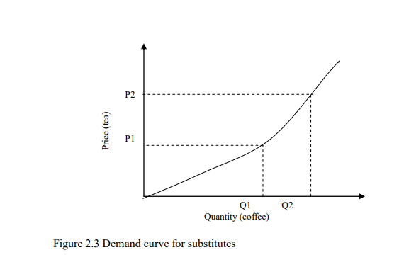
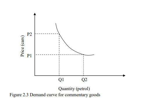
Two goods, X and Y are said to be substitutes if a rise in the price of one commodity, say Y, leads to a rise in the demand of the other commodity X. If the price of tea increases consumers will find coffee relatively cheaper to tea as a result demand for coffee increases. Substitutes are commodities that can be used in place of other goods. This phenomenon is illustrated in Figure 2.3. The graph shows the relationship between the prices of tea over the quantity for coffee. If the price of tea increases from P1 to P2 the quantity of coffee demanded increases from Q1 to Q2.
Compliments goods such as shoe and polish, pen and ink cars and petrol, computers and software, bread and margarine, hamburgers and chips, tapes and tape recorders. Demand for some commodities can also be affected by changes in the prices of the complementary if a rise in the price of one of the goods, say A leads to the fall in the demand of another food, say B. Complimentary goods are usually jointly demanded in the sense that the use of one requires or is enhanced by the use of the other. Figure 2.4 illustrates the relationship between complementary goods graphically. For example if the price of cars is lowered demand for petrol increases because more cars will be bought/demanded. The curve shows the relationship between the price and of a car and quantity demanded for petrol. If the price of cars falls from P2 to P1 the quantity demanded for petrol increases from Q1 to Q2.
Changes in disposal real income. An individual’s level of income has an important effect on the level of demand for most products. If income increases demand for the better quality goods and services increases. This relationship however, depends on the type of goods and level of consumers‟ income. The three types of are goods; Normal gods these are goods whose demand increases as income increases. The demand for normal goods increases continuously with increase in income. It tends to become gently as people reach the desired level of satisfaction.
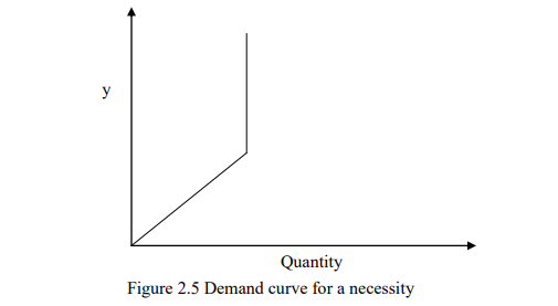
Inferior goods refer to goods for consumers with low income levels such that as income increases its demand falls. At low level of income, these individuals will tend to consume large amount of these goods but as income increases they buy other goods which they consider superior thus demanding less of the inferior goods. At very low level of income an inferior good behave like a normal good only to behave inferior as income increases. Necessities these are goods which consumers cannot do without such as salt, match boxes among others. Their income demand curve tends to remain constant other than at the lowest levels of income as indicated in Figure 2.5
Changes in consumer tastes, preferences and fashion Personal tastes play an important role in governing the consumer’s demand for certain goods. For example, preferring to consume imported commodities despite them being extremely expensive. Prevailing fashions are an important determinant of tastes. The demand for clothing for example, particularly is susceptible to changes in fashion.
Level of advertising is also an important determinant of demand. In highly competitive markets, a successful advertising campaign will increase the demand of a particular product while at the same time decreasing the demand for competing products. Increase in advertising will increase demand in the following ways;
- it helps inform about the product of a firm
- Can introduce new products to the market.
- Induce individuals to frequently use the product/service
Factors affecting advertising policies
- cost of advertising
- mode of advertising
- impact of advertising on the demand of the product
- The target group (old, young)
- number of competitors and quality of their products
- The market share of the firm and the degree of competition
- Future expectations in price changes
- Government policies and taxes
- Appropriate time to make advertisements
- Cultural background
- Language
The availability of credit consumers. This factor especially affects the demand for durable consumer goods which are often purchased on credit. For example a decrease in availability of credit or the introduction of more stringent credit terms is likely to lead to a reduction in the demand of some durable consumer goods. The government policy The government may influence the demand of a given commodity through legislation. For example making it mandatory for everyone to wear seatbelts. The consumers inevitably get to purchase more seatbelts as a result. Subsidies it’s the opposite of taxation. When the government grants subsidies prices
of goods falls leading to increase in demand and vice versa. Climate change demand of various goods varies depending on weather. For instance there is high demand for woolen clothes during rainy reasons
2. Market factors affecting individual demand
It’s a horizontal demand sum of the demands for individual consumers. It refers to quantity demanded in the market at each price by individual consumers. For this reason all the factors affecting individual demand will affect market demand. The market demand for a commodity can be derived graphically as in Figure 2.6.
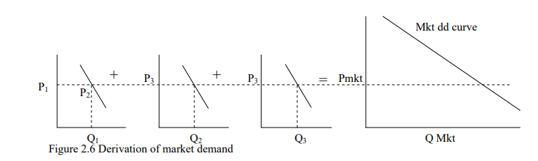
Where P1, P2 and P3 are individual prices Q1, Q2 and Q3 are individual quanties demanded. Pmk is the market price qmk is market quantity demanded.
Other factors affecting market demand
Change in population market demand is influenced by the size of the population, the composition of the population in terms of age sex as well as geographical distributions. Distribution of income more evenly distribution of income may increase demand for
normal goods while at the same time it may lower the demand for luxuries.
2.3 Movement Along and Shift in Demand Curve
Demand is a multi- variant function in the sense that it is influenced by so many factors such as the price of the commodity, the price of other related commodities, consumer incomes etc. The price of the commodity is the most important determinant of demand and its relationship with the quantity demanded give rise to a demand curve. Movement along demand curve is demonstrated by a change in the price of a good as shown in Figure 2.7 by movement from one point to another on the same demand curve.
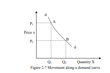
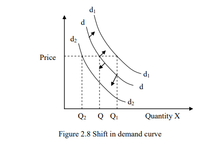
A change in price of a good from P1 to P2 causes a movement from point A to B along the demand curve. This movement along demand curve shows a change in quantity demanded which is an increase or a fall in the quantity demanded. A shift in the demand curve is caused as a result of a change in any factor affecting demand other than price such as changes in consumer income tastes and preferences. For this reason all other factors affecting demand other than price of the product are also referred to as shifting factors as illustrated in Figure 2.8 Any change in the shifting factors will cause changes in demand (an increase or a fall in demand). A shift to the right (dd to d1d1) shows an increase in demand while a shift from (dd to d2d2) shows a decrease in demand.
Terms used in demand
- Joint demand it is the demand whereby two commodities are always demanded together. One good cannot be demanded in the absence of the other such as car and petrol.
- Competitive/rival goods it is the demand for goods which are substitutes such tea and coffee.
- Derived demand where goods are demanded in order to provide goods such as cotton is required to produce cotton wool
- Composite demand (several uses) where some goods are used for different purposes such as steel for cars machine etc
2.4 Definition of Supply
Individual supply refers to the quantity of a given commodity that a producer is willing and able to sell at a given price over a specific time period. Market supply refers to horizontal summation of individuals producers/firms supply in the market. The supply schedule and the supply curve demonstrate the relationship between market prices and quantities that suppliers are willing to offer for sale. Supply differs from “existing stock” or the amount available because it is concerned with amounts actually brought to the market. The basic law of supply states that, “a greater quantity will be supplied at a higher price than at a lower price”. An individual producer’s supply schedule shows alternative quantities of a given commodity that a producer is willing and able to sell various alternative prices for that commodity ceteris paribus (other things remaining constant).
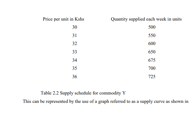
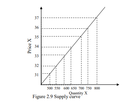
A supply curve show the relationship between the price of the commodity and the quantity supplied. The relationship is a direct one as the supply curve slopes upwards from left to right. The direct relationship is a graphical representation of the law of supply which states that other things remaining constant a greater quantity will be supplied at higher prices and vice versa.
Determinants of Supply
The supply of a good is influenced by the following factors
- price of the commodity in the market
- the price of other related goods
- cost of production
- state of technology
- objective of the firm
- future expectations of price changes
- climate
- government policy and taxes
Price of the good as the price of a given commodity say X rises, with the costs and the prices of all other goods remaining unchanged, the production of commodity X becomes more profitable. The existing firms are therefore likely to expand their profit and new firms are to be attracted into the industry. It should be noted however, that not just the current rise but also expectations concerning the future increases prices may motivate producers. The total supply of goods is expected to increase as the prices rise. Prices of other related goods changes in the prices of other commodities may affect the supply of a commodity whose price does not change.
Substitutes; two goods X and Y are said to be substitutes in production if the supply of good X is inversely/negatively related to the price of Y. For instance barley and wheat or tea and coffee. If a firm producing both tea and coffee notices that the price of tea is rising may decide to allocate more resources to tea at the expense of coffee. The supply of coffee will therefore fall as the price of tea increases. However, the movement of resource from one use to the other is dependent on the mobility of factors of production.
Complimentary goods; two goods X and Y are said to be compliments if an increase in the price of X causes an increase in the supply of Y such as a vehicle and petrol. Jointly supplied goods; two goods X and Y are said to be jointly supplied if an increase in the price of X causes an increase in the price of Y such as petrol and paraffin. If the demand for petrol increases the supply of petrol will rise and at the same time the supply of paraffin will increase.
N/B The extent to which firms can move from one industry to another in search of higher profits depends on occupational and geographical mobility of the factors of production.
Prices of factors of production as the prices of factors of production used intensively by producers of a certain commodity rise, so do the firm costs. This will cause the supply to fall since some firms will eventually leave the industry. Similarly, if the price of one factor of production, say land, increases, some firms may move out of the production of land intensive products into the production of goods that are intensive in other factors of production which are relatively cheaper. Finally other less efficient firms will make losses and eventually leave the market.
The state of technology is a society’s pool of knowledge concerning industrial activities and its improvements. Technological improvements or progress such as improvements in machine performance, management and organization or an improvement in quality of raw materials leads to lower costs through increased productivity and increases the profit margin in every unit sold. This leads to increase in supply.
Future expectations of price change Supply of a good is not only influenced by the current prices but future expected price as well. For example, if the price of a good is expected to rise the firm may decide to reduce the amount of supply in the current period. This is to enable them pile stock which they can offer for sale when prices increase in the future. This is known as hoarding. Government policies through tax imposition on goods increases the cost of production hence decline in production and supply Through subsidies -a grant to citizens of a country which lowers the cost of production hence encourages production and increases in supply.
Through price control can either by price minimization where prices are fixed above equilibrium encouraging producers to produce more hence increase in supply. It may be undertaken through price maximization where prices are fixed below equilibrium discouraging production hence decline in supply. Though quotas where the government puts restriction or limit production of various goods which leads to decline in supply. Weather /climate the supply of agricultural products is considerably affected by changes in weather conditions. Output in agriculture is subject to variations in weather from year to the next. An excellent growing season associated with favorable weather conditions will result in a bumper harvest leading to an increase in supply. An unfavorable season that results in a poor harvest may be viewed as an increase in the average costs of production because a given expenditure on inputs yields a lower input than it would in a good/ favorable season. A bad harvest is represented by a leftward shift of the supply curve.
Objectives of the firm a business may pursue several objectives such as sales maximization, market leadership, quality leadership, survival, profit maximization, social responsibility. Firms with sales maximization as an objective aim at supplying greater quantities of its product than a firm aiming at profit maximization where the later supplies less quantities but at a higher price in order to maximize the profit. Incidence of strikes lead to a reduction in supply of a product. The supply of manufactured goods is particularly likely to be affected by industrial disputes because of generally stronger unions in the industrial sector.
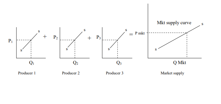
Market supply
The market supply curve represents the alternative amount of a good supplied per period of time at various alternative prices by all the producers of goods in the market. The market supply of goods therefore will be influenced by all the factors that determine individual producer supply and all the number of producers of goods in the market. This concept is illustrated in Figure 2.10 It therefore follows that the market supply curve will have a gently slope than individual supply curves. Figure 2.10 Derivation of market supply curve
2.5 Movement Along and Shift in Supply Curve
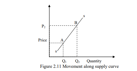
The relationship between price of a commodity and quantity supplied give rise to a supply curve. Any changes in the price of a good causes change in the quantity supplied. This can be traced by the movement along supply curve as shown in Figure 2.11 The movement from point A to B is caused by changes in price from P1 to P2 which bring fourth the movement along the supply curve.
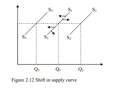
A shift of supply curve is caused by a change in any other factors affecting supply other than the price of the goods. This shift indicates changes in supply as a result of e.g. advances in technology which makes it cheaper to produce goods and services and therefore their supply will increase. Similarly incase of increase in cost of production will lead to a fall in quantity supplies as shown in Figure 2.12. A shift to the right from S1S1 to S3S3 shows a fall in supply.
2.6 The Concept of Equilibrium in Economics
Equilibrium in economics refers to a situation in which the forces determine the behavior of variables are in balance and therefore exert no pressure on these variables to change. In equilibrium the actions of all economic agents are mutually consistent. Market
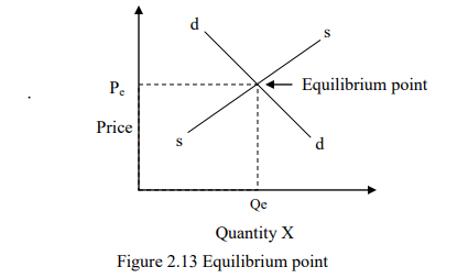
equilibrium occurs when the quantity of a commodity demanded in the market per unit equals the quantity of the commodity supplied to the market over the same period of time. Geometrically, equilibrium occurs at the intersection point of the commodity’s
market demand and market supply curve. The price and quantity at the equilibrium are known as the equilibrium price and equilibrium quantity respectively. The price Pe is also referred to as market clearing point. At this equilibrium point the amount that producers are wiling and able to supply in the market is just equal to the amount that consumers are wiling and able to demand. Both consumers and producers are satisfied and there is no pressure on prices to change and thus the market for goods is said to be at equilibrium. This is illustrated in Figure 2.13 Equilibrium point
Equilibrium can be defined as a state of rest or balance in which no economic forces are being generated to change the situation. These economic forces are excess demand and supply and are illustrated in Figure 2.14. At P1, the quantity demanded by consumers is
Q1 units but producers are willing to supply at price a quantity of Q2 units. Therefore there is an excess supply equal to (Q2 –Q1). Excess supply refers to a situation where quantity demanded is less than quantity supplied at prevailing market price. Producers
may therefore react to the excess supply by lowering prices of their products so as to sale the unsold stocks. Excess supply is referred to as a buyer’s market since suppliers may be obliged to lower their prices in order to dispose of excess output a situation which is
favorable to buyers. Excess supply represents an economic force that exerts downward pressure on prices. At P2 the quantity demanded is Q2 but producers are wiling to supply Q1 units of goods. Therefore, there will be excess demand equal to (Q2-Q1). This
situation of excess demand is referred to as sellers market because competition among buyers will force up the price due to the existing shortage Excess supply is a situation where quantity demanded is greater than quantity supplied at prevailing market prices.
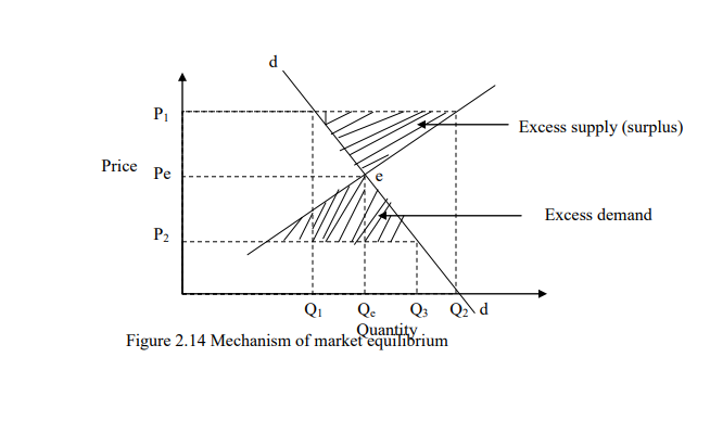
In this case, the price of goods will rise because of competition among buyers. Excess demand represents an economic force on prices which exerts upward pressure. Prices P1 and P2 are disequilibrium prices and market is said to be at disequilibrium. Therefore, the
general rule for equilibrium is that demand should equal supply represented by Qe and Pe.
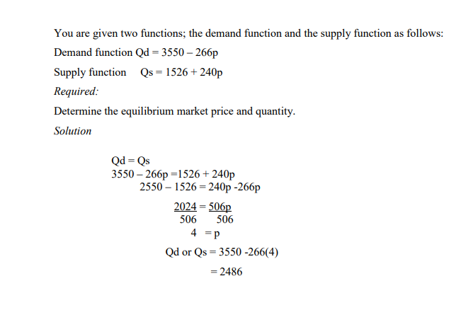
2.6.1 Mathematics Derivation of Equilibrium
Exercise 2.1
2.6.2. Types of Equilibrium
The are three types of equilibrium; stable, unstable and neutral.
1. Stable equilibrium If there is a force that distracts market equilibrium then there will adjustment that brings back the prices and quantity demand to the initial equilibrium. This is well explained in the previous section.
2. Unstable equilibrium equilibrium is said to be equilibrium if there is divergence from the equilibrium set by forces which push the prices further away from the equilibrium prices. For example, in case of a giffen good which assumes a demand curve which is positive as indicated in Figure 2.15
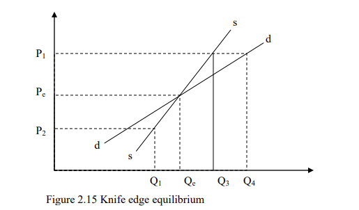
At P1 there is excess demand and this will exert an upward pressure on the prevailing market thus push it further away from the equilibrium. At p2 there is excess demand and this will exert an upward pressure on the prevailing market prices thus pushing it further away from the equilibrium. This type of equilibrium is known as knife edge equilibrium. A small in price will send the system further away from the equilibrium.
3. Neutral equilibrium occurs when initial equilibrium is disturbed and forces of disturbances leads to a new equilibrium point. It may occur due to a shift of either demand or supply or through the effect of taxes.
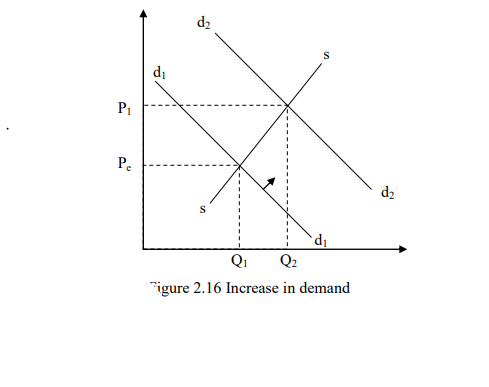
The effect of a shift of demand and supply on market equilibrium.
Shift in demand
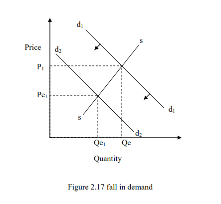
Increase in demand. Consider Figure 2.16 which illustrates the effect of an increase on demand on market equilibrium. An increase in demand is represented by a shift of the demand curve from d1d1 to d2d2. The immediate effect will be shortage and this will force prices to rise leading to increase in quantity supplied until equilibrium is reestablished at Pe. Fall in demand Consider Figure 2.17 which illustrates the effect of a fall in demand on the market equilibrium.
A fall in demand is represented by a shift of demand curve to the left from d1d1 to d2d2. The immediate effect will be a surplus and this will force the producers to lower the price in an attempt to get rid of excess stock. This fall in price will led to decline in quantity supplied until a new equilibrium is established at Pe1; Qe1
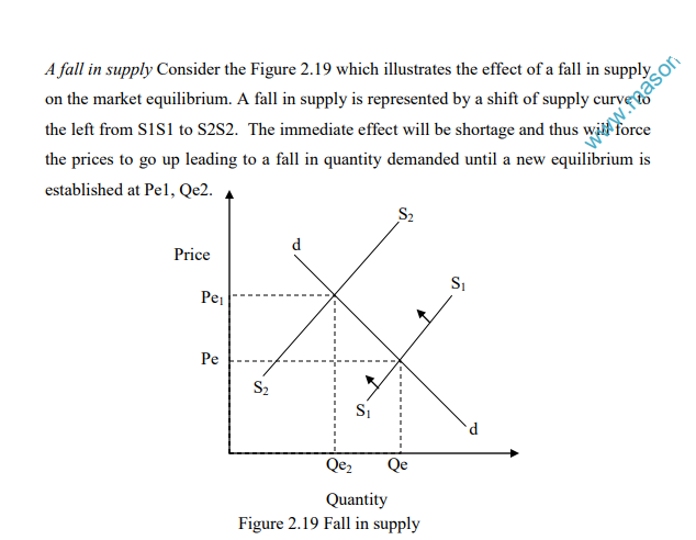
Shift in supply
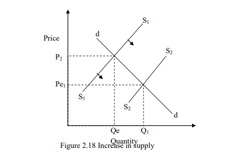
Increase in supply Consider Figure 2.18 which illustrates the effect of an increase of supply on the market equilibrium. An increase in supply is represented by a shift of supply curve to the right from S1S1 to S2S2. The immediate effect will be surplus and this will force the producer to lower their prices in order to get rid of excess stock. This fall will lead to an increase in quantity demanded until a new equilibrium is established at Pe.
2.7 Price Control
This refers to a deliberate action by the government to artificially impose through legislation the prices of certain goods and services. Such imposed prices are referred to as flat prices. These flat prices may be a maximum or a minimum price. A maximum price refers to that price above which a good or a service cannot be sold. A minimum price refers to that price below which a good/service cannot be sold. The government may find it necessary to control the prices of certain good/service because:
- Cheapness It may be objective of the government to keep price of certain goods and services at a level at which they can be afforded by most people hence protecting the consumer being exploited by producers
- Maintenance of income. The government may want to keep the income of certain producers at a higher level than that which would be supplied by market forces demand and supply. Thus the government is able to maintain the low income producers in the market.
- Price stability if there is a wide variation in the price of product year to year the government may wish to iron out these variations for the interests of both producers and consumers. This price control will act as one of the methods to curb inflation.
Advantages of price control
- Protects consumers, especially the low income consumers from price increases by producers.
- Ensures that producers have a reasonable income which is subject to inflation
- Contributes to industrial peace especially if they constitute part of the comprehensive income policy and a maximum price is fixed on some basic goods.
- It may be associated with a decrease in price and an increase in output such as the case of a monopolist overcharging for its products and is forced to lower prices. In this case the monopolist may accompany the fall in price with an increase in
output in order to compensate for loss in revenue. - It may be used as one of the several counters of inflation.
2.8 Elasticity of Demand
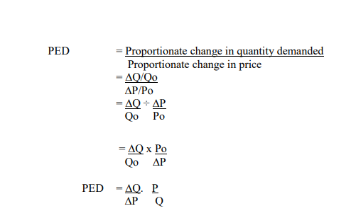
It can be defined as the ratio of the relative change of a dependent variable to changes in another independent variable. Elasticity can be analyzed in terms of demand and supply. It can also be defined as a measure of responsiveness of quantity demanded of a good in
to changes in income or prices of other related goods. There are three types of elasticity; price elasticity of demand, cross elasticity of demand and income elasticity of demand. Price elasticity of demand it’s the measure of responsiveness of the quantity demanded of
a commodity to changes in its own price. It is also referred to as own price elasticity. It abbreviated as PED/ED. It is calculated as follows
2.8.1 Types of elasticity
There are five types of elasticity of demand.
- Perfectly elastic demand. Demand is said to be perfectly elastic when the consumers are willing to buy an amount of a commodity at a given price, but non at a slightly higher price.
- Elastic demand. Demand is said to be price elastic when a charge in price causes more than proportionate change in quantity demanded.
- Unity elastic demand. Demand is said to unit elastic if changes in price cause proportionate change in quantity demanded. If price increase quantity falls in the same proportion and vice versa.
- Inelastic demand. Demand is said to be price inelastic if changes in price causes less than proportionate change in quantity demanded. If prices increases the quantity falls in less proportion and if the prices falls the quantity demanded increases in less proportion ED < 1
- Perfectly inelastic demand. Demand is said to be perfectly price inelastic if changes in price has no effect on the quantity demand (ED= 0).
Factors affecting price elasticity of demand
- Substitutability. If a substitute is available in the relevant price range, quantity demanded will be elastic. The demand for a particular brand of cigarettes maybe considered being elastic because if there is existence of other brands that are close
substitutes. However, the total demand for cigarettes may be inelastic because there are no close substitutes for cigarette. It can hence be said that the greater the number of substitutes for a given commodity, the greater will be its price
elasticity of demand. - The proportion of a consumer’s income spent on the commodity. If this proportion is very small as in the case of match boxes , the quantity demanded will tend to be inelastic. On the other hand if this proportion is relatively large as for example in the case of meat, demand will tend to be elastic. This implies that the greater the proportion of income which the price of the product represents, the greater price elasticity of demand will end to be.
- The extent to which the product is habit forming. Habit forming products like cigarettes or alcohol have a low price elasticity of demand. In the case of in addiction to, say drugs, the price elasticity of demand is likely to be even lower.
- The number of uses of a commodity. The greater the number of uses of the commodity, the greater the price of elasticity. The elasticity of alluminium for example is likely to be much greater than of butter because butter is mainly used as food while alluminium has hundreds of uses such as electrical wiring and appliances.
- The length of adjustments. The longer the period allowed for adjustment in the quantity demanded as a commodity the greater its price elasticity is likely to be. This is because it usually takes some time for new prices to be known and for consumers to make the actual switch. Consumers adjust buying habits slowly.
- The level of prices. If the ruling price is at the upper end of the demand curve, quantity demanded is likely to be more elastic than if it was towards the lower end. This is always true for a negatively sloped straight line demand curve.
- Necessities and luxuries Demand for luxury is likely to be price elastic while the demand for necessities is generally price inelastic. However, this depends with availability of close substitutes.
- Width/size of the market the wide definition of the market of a good, the lower is the price elasticity of demand. Thus for wide markets demand will tend to be price inelastic while for a small market demand will tend to be price elastic.
- Time demand for most goods and services tend to be more elastic in the long run as compared to the short run period. This is because consumers will take some time to respond to price changes. For instance, if the price of petrol falls relative
to diesel, it will take long for motorists to respond because they are locked in existing investment in diesel engines. - Durability of the commodity durable goods have low elasticity of demand or they are price elastic while perishable goods are price inelastic.
Importance of price elasticity of demand/economic application of the concept of elasticity
- The consumer needs knowledge of elasticity when spending income where more income is spent on goods whose elasticity of demand is inelastic and vice versa.
- The government imposes taxes with inelastic demand and vice versa. Devaluation when a country devalues or lowers the value of its currency. The currency is made cheaper relative to other currencies. This makes a country’s exports cheaper for foreigners. Its import expensive for the residents. For a country to benefit by increasing exports, the elasticity of demand must be high.
- Business/producers They use elasticity of demand on deciding on whether to charge high or lower prices or even deciding on commodities to bring to the market especially those which are price inelastic.
Importance of Income Elasticity of Demand
- Business firms- if demand of a commodity is elastic to price, its possible to revenue by reducing prices. Businesses use specific information to know which price to increase to eliminate shortages or which price to reduce to eliminate surpluses.
- Government uses elasticity to determine the yield of indirect taxes. Inelastic commodities are highly taxed. However, if demand of a commodity is elastic an increase in tax will hinder production
- Price elasticity is relevant for a country considering devaluation as a means of rectifying balance of payment disequilibrium. Devaluation decreases imports and increases exports. However, this will depend on demand of import and export elasticities.
- It helps to explain price instabilities in the agricultural sector
- Monopolists apply price discrimination by understanding the demand elasticities. High price is charged to those markets with lower price elasticity
Factors affecting Income elasticity of demand
- Nature of the need that the commodity covers. For certain goods and services the percentage of income spent declines as income increases such as food.
- The initial level of income of a country (level of development) TV sets, refrigerators, motors vehicles are considered as luxuries in underdeveloped countries while they are considered as necessities in countries with high per capita income.50
- Time period. The demand for most goods and services will tend to be income elastic in the long run as compared to short run period. This is because the consumption pattern adjusts with time and also with change in income.
Type of price elasticity of supply
1. Perfectly elastic supply
2. Elastic supply
3. Unit elastic supply
4. Inelastic supply
5. Perfectly inelastic supply.
Factors affecting price elasticity of supply
- Mobility of factors of production If they are highly mobile then supply will be price elastic since more factors can be employed quickly when the prices increase thus increase in supply
- The level of employment of resources It refers to the utilization and allocation of resources. If the factors are fully utilized supply will be price inelastic due to the fact that all the facts are occupied and thus can not be mobilized in order to increase supply. However if they are under employed, supply will be price elastic.
- Production period for product that take short period of time to produce their supply tend to be price elastic. While thus that take a longer period will be price inelastic because it will take a while before the products can reach the market.
- Nature of the commodity Price elasticity of supply for perishable goods tend to be inelastic due to the fact that the goods do not respond to price fall as they can not be easily stored. On the other hand supply for durable goods tend to be price elastic since they can be store when the price falls thus contracting supply.
- Risk taking If the entrepreneurs are willing to take risk then supply of the products will be price elastic. Risk taking will in return be determined by the prevailing conditions in the economy. E.g. Political stability, security, government incentives, infrastructure, etc.
- Level of stock If it‟s high supply will be price elastic because if the price of a good increases more of the good will is supplied from the stock
- Time period Supply for most goods and services will tend to be more elastic in the long run than in the short run because producer need more time to reorganize factors of production so that they can increase supply of the products.
Importance of price elasticity of supply
- If supply of a good is price elastic thus an increase in demand will benefit both the producer and consumer of products because the producer will be in apposition to supply relatively more of their products and consumer will eventually pay a relatively lower price.
- If the supply of commodity I price inelastic business may risk losing revenue when there is a fall in the price of their products. This is because they will be forced to sell their products at a loss or a reduced price margin, e.g. In the case of perishable goods, however in the supply of the goods is price elastic the business people may store their products when price fall thus contracting
supply e.g. the case of durable goods.
Relationship between total revenue and elasticity
- Elastic demand Increase in price will reduce the total revenue while a fall in price increase the total revenue
- Inelasticity demand Increase in price will reduce the total revenue while a fall in price causes reduction in total revenue.
- Unit demand change in price will leave the price unchanged.
Application of elasticity in economic policy decisions
- Products/services pricing decisions
- Customer spending programmes
- Production decisions
- Government policy orientation -Taxation policy
Evaluation policies
Price control/minimum - Price discrimination
- Shift of the tax burden