
6.0 Analysis and Presentation of Data
Once the data begin to flow in, attention turns to data analysis. The steps followed in data collection influence the choice of data analysis techniques. The main preliminary steps that are common to many studies are:
- Editing
- Coding and
- Tabulation
Editing
Editing involves checking the raw data to eliminate errors or points of confusion in data. The main purpose of editing is to set quality standards on the raw data, so that the analysis can take place with minimum of confusion. In other words, editing detects errors and omissions, corrects them when possible and certifies that minimum data quality standards are achieved. The editor’s purpose is to guarantee that data are:
• Accurate
• Consistent with other information
• Uniformly entered
• Complete and
• Arranged to simplify coding and tabulation.
In the following questions asked of military officers, one respondent checked two categories, indicating that he was in the reserves and currently serving on active duty.
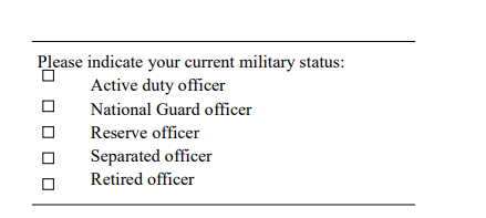
The editor’s responsibility is to decide which of the responses is consistent with the intent of the question or other information in the survey and is most accurate for this individual respondent.
There are two stages in editing:
- the field edit
- the central office edit
The Field Edit
Field edit is the preliminary edit whose main purpose is to detect the obvious inaccuracies and omissions in the data. This also helps the researcher to control the fieldworkers and to clear misunderstandings of the procedures and of specific questions.
The best arrangement is to have the field edit conducted soon after the data collection form has been administered. The following items are checked in the field edit:
- Completeness: Checking the data form to ensure that all the questions have been answered. The respondent may refuse to answer some questions or may just not notice them.
- Legibility: A questionnaire may be difficult to read owing to the interviewer’s handwriting or the uses of abbreviations not understood by respondents.
- Clarity: A response may be difficult for others to comprehend but the interviewer can easily clarify it, if asked in good time.
- Consistency: The responses provided may also lack consistency. These can be corrected by the fieldworker if detected early.
In large projects, field editing review is a responsibility of the field supervisor. It, too, should be done soon after the data have been gathered. A second important control function of the field supervisor is to validate the field results. This normally means s/he will re-interview some percentage of the respondent, at least on some questions.
Central Editing
This comes after the field edit. At this point, data should get a thorough editing. Sometimes it is obvious that an entry is incorrect, is entered in the wrong place or states time in months when it was requested in weeks. A more difficult problem concerns faking; Arm chair interviewing is difficult to spot, but the editor is in the best position to do so. One approach is to check responses to open-ended questions. These are the most difficult to fake. Distinctive response patterns in other questions will often emerge if faking is occuring. To uncover this, the editor must analyse the instruments used by each interviewer.
2. Coding
It involves assigning numbers or other symbols to answers so the responses can be grouped into a limited number of classes or categories. The classifying of data into limited categories sacrifices some data detail but is necessary for efficient analysis. Instead of requesting the work male or female in response to a question that asks for the identification of one’s gender, we could use the codes ‘M’ or ‘F’. Normally, this variable would be coded 1 for male and 2 for female or 0 and 1. Coding helps the researcher to reduce several thousand replies to a few categories containing the critical information needed for analysis.
The first step involves the attempt to determine the appropriate categories into which the responses are to be placed. Since multiple choice and dichotomous questionnaire have specified alternative responses, coding the responses of such questions is easy. It simply involves assigning a different numerical code to each different response category.
Open questions present different kinds of problems for the editors. The editor has to categorise the responses first and then each question is reviewed to identify the category into which it is to be placed. There is a problem in that there can be a very wide range of responses, some of which are not anticipated at all. To ensure consistency in coding, the task of coding should be apportioned by questions and not by questionnaires. That is, one person may handle question one to six, in all the questionnaires instead of dividing the coding exercise by questionnaires.
The next step involves assigning the code numbers to the established categories. For example, a question may demand that a respondent lists the factors s/he considers when buying a pair of shoes. The respondent is free to indicate anything s/he thinks of. The responses may range from colour, size, comfort, price, materials, quality, durability, style, uniqueness and manufacturer among others. The response may have to be coded into just three or four categories and each response has to be placed within a specific category and coded as such. The ‘don’t know’ (DK) response presents special problems for data preparation. When the DK
response group is small, it is not troublesome. But there are times when it is of mjaor concern, and it may even be the most frequent response received. Does this mean the question that elicited this response is useless? It all depends. But the best way to deal with undesired DK answer is to design better questions at the beginning.
3. Tabulation
This consists of counting the number of responses that fit in each category. The tabulation may take the form of simple tabulation or cross tabulation.
• Simple tabulation involves counting a single variable. This may be done for each of the variables of the study. Each variable is independent of the others.
• In gross tabulation two or more variables are handled simultaneously. This may be done by hand or machine.
Where hand tabulation is used, a tally sheet is used. For example, if the question read: How many cigarettes do you smoke in a day?
The tally for a sample of size 35 would look like this:
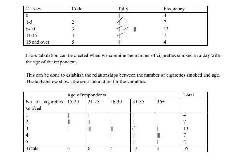
The cross tabulations indicate for example, that all the respondents smoking more than 5 cigarettes a day are in the 36 and over years of age category. This kind of tabulation is only useful in very simple studies involving a few questions and a limited number of responses. Most studies involve large numbers of respondents and many items to be analysed and these generally rely on computer tabulation. There are many packaged programmes for studies in the social sciences.
A note on the use of summary statistics
Researchers frequently use summary statistics to present survey findings. The most commonly used summary statistics include:
Measures of central tendency (mean median and mode).
Measures of dispersion (variance, standard deviation, range, interquartile range).
Measures of shape (skewness and kurtosis).
We can also use percentages.
These are all summary statistics that are only substitutes for more detailed data. They enable the researchers to generalise about the sample of study objects. It should be noted that these summary statistics are only helpful if they accurately represented the sample.
One can also use some useful techniques for displaying the data. These include frequency tables, bar charts, and piecharts, etc.
6.1 Hypothesis Testing
There are two approaches to hypothesis testing. The more established is the classical or sampling theory approach; the second is known as the Bayesian approach. Classical statistics are found in all of the major statistics books and are widely used in research applications. This approach represents an objective view of probability in which the decision making rests totally on an analysis of available sampling data. A hypothesis is established, it is rejected or fails to be rejected, based on the sample data collected.
In classical tests of significance, two kinds of hypothesis are used:
- The null hypothesis denoted Ho; is a statement that no difference exists between the parameter and the statistic being compared.
- The alternative hypothesis denoted H1; is the logical opposite of the null hypothesis. The alternative hypothesis – denoted (H1) may take several forms, depending on the objective of the researchers. The H1 may be of the ‘not the same’ form (nondirectional). A second variety may be of the ‘greater than’ or ‘less than’ form (directional).

Note:
A type I error is committed when a true hypothesis is rejected and a type II error is committed when one fails to reject a false null hypothesis.
Statistical Testing Procedures:
- State the null hypothesis.
- Choose the statistical test.
- Select the desired level of significance. ∝ 0.05 ∝ 0.01.
- Compute the calculated difference value.
- Obtain the critical test value, ie, t, z, or x2
- Make the decision. For most tests if the calculated value is larger than critical value, we reject the null hypothesis and conclude that the alternative hypothesis is supported (although it is by no means proved).
A Note on Tests of Significance
There are two general classes of significance tests, parametric and nonparametric.
• Parametric tests are more powerful because their data are derived from interval and ratio measurements.
• Nonparametric tests are used to test hypothesis with nominal and ordinal data.
Parametric Tests
The Z or t test is used to determine the statistical significance between a sample distribution mean and a parameter. The Z distribution and t distribution differ (the latter is used for large samples, ie, greater than 30). But when sample sizes approach 120, the sample standard deviation becomes a very good estimate of the population standard deviation; beyond 120, the t and Z distributions are virtually identical.
One-Sample Tests:
These are used when we have a single sample and wish to test the hypothesis that it comes from a specified population. In this case, we encounter questions such as these:
- Is there a difference between observed frequencies and the frequencies we would expect, based on some theory?
- Is there a difference between observed and expected proportions?
- Is it reasonable to conclude that a sample is drawn from a population with some specified distribution (normal, poison, and so forth)?
- Is there significant difference between some measure of central tendency (x) and its population parameter (u)?
Notes:
- It is important to realise that if the null hypothesis is accepted, this is not proof that the assumed population mean is correct. Testing a hypothesis may only show that an assumed value is probably false.
- It will be apparent from the two examples that the 1% level of significance is a more severe test than the 5% level. The greater the level of significance, the greater the probability of making a Type I error.
Non-Parametric Tests
Probably the most widely used non-parametric test of significance is the chi-square (x2) test.
This test does not make any assumption about the distribution from which the sample is taken. The x2 test is an important extention of hypothesis testing and is used when it is wished to compare an actual, observed distribution with a hypothesised or expected distribution. It is often referred to as a ‘goodness of fit’ test.
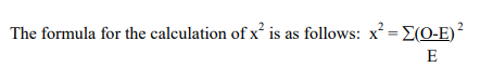
Where O = the observed frequency of any value.
E = the expected frequency of any value.
Procedure:
1. Null hypothesis Ho : O = E
H1: O ≠ E
2. Statistical test: Use the one-sample x2
to compare the observed distribution to a hypothesized distribution.
3. Significance level: ∝ = 0.05 or 0.01.
4. Calculated value:
![]()
5. Critical test value: Locate the table critical values of x2
6. Decision: If the calculated value is greater than (less than) the critical value, reject null hypothesis (accept Ho).
6.2 Introduction Comments on Correlation and Regression Analysis
Correlation and regression analysis are complex mathematical techniques for studying the relationship between two or more variables. Correlation analysis involves measuring the closeness of the relationship between two or more variables. Regression analysis refers to techniques used to derive an equation that relates the dependent variable to one or more independent variables. The dependent variable here refers to the variable being predicted. The independent variables are those that form the basis of the prediction – they are also called predictor variables
Correlation and regression techniques may be used in situations where both the dependent and independent variables are of the continuous type. When a survey data consists of a continuous dependent variable and one or more continuous independent variables, researchers may use the techniques of correlation and regression analysis.
A straight line is fundamentally the best way to model the relationship between two continuous variables. The bivariate linear regression may be expressed as: Y = β0 + β0XI Where the value of the dependent variable Y is a linear function of the corresponding value of the independent variable (X)