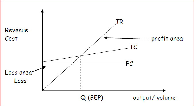
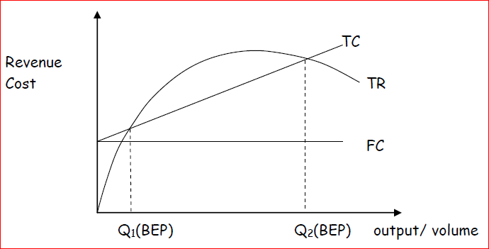
This is a systematic way of examining the relationship between changes in activity level and changes in the total sales revenues, expenses and net profit. The objective of CVP analysis is to establish what would happen to the financial results if a specified activity level or volume fluctuates. This information is important to the management because volumes or output is the major variable influencing the sales revenue, total cost and profit. CVP analysis is also called Break Even analysis and can be represented graphically.
The accountants assume that total revenue and total cost are linear functions of output. There is therefore only one BEP. The optimal volume is thus the maximum possible volume that can be accommodated by the available production infrastructure.

Economists assume that total revenue is a curvilinear function of output. They believe that the business can only sell increasing quantities of the product if they lower the prices. This gives rise to two break even points. The optimal volume is therefore at the point where the difference between the TR curve and the TC curve is largest.

Difference between the accountant’s and economist’s model of the C-V-P
Accountants’ model of the C-V-P
Accountants argue that the breakeven point is the point where the total revenue is equal to the total costs (TR=TC). Accountants assume that variable
cost and selling price per unit are constant at all levels. This results in a linear relationship for the total cost, total revenue and profit. In this view
therefore, there will only be one break-even point (BEP) and the profit area widens as sales volume increases
Economists’ model of the C-V-P
Economists argue that the breakeven point is the point where marginal revenue is equal to the marginal costs. Economists assume that the C-VP
functions are non-linear or curvilinear due to the economies and diseconomies of scale e.g. to increase the total revenue the business entity can
increase the quantity of output by reducing selling price per unit.
General assumption of CVP analysis
- Variable cost per unit is assumed to remain constant.
- Selling price per unit is assumed to remain constant.
- The fixed cost is assumed to be constant within the relevant range.
- The total cost and total revenue are assumed to be linear functions output.
- Costs can accurately be divided into their variable and fixed component.
- The analysis applies in the short term time horizon only.
- Production quantity equals to sales quantity i.e. there are no stocks.
- It assumes a single product or a constant sale mix in the case of multiple products.
THE CVP MODEL
Net profit = Total revenue – Total cost
Therefore net profit = Total revenue – total variable cost – total fixed cost
Assume the following notations: NP = net profit Q = the volume (output/sales quantity) p = selling price per unit a = Total fixed cost b = Variable cost per unit Therefore NP= Q(p-b)-a
Therefore net profit = total revenue – total variable cost – total fixed cost
NP = Qp – Qb-a
At BEP, the NP = Zero;
0 = Qp –Qb-a
Limitations of C- V- P analysis
- Fixed costs can only remain fixed within the relevant range and cannot therefore be constant when the firm operates outside the relevant range.
- Costs cannot be entirely classified between variable and fixed because there are always costs that have characteristics of both
- The selling price and variable cost per unit cannot remain constant because the firm may offer discounts to customers while variable costs may increase due to inflation, or reduce due to discounts from suppliers.
- The firm will not always produce units using the same technology and therefore changes are always anticipated in the production process which changes will affect the operating capacity of the firm. The firm can either produce more than or less than the budgeted units.
- C- V- P analysis is a single product model and cannot be used where a firm has several products.
- A firm will always have opening and closing inventories because production cannot be equal to sales.

