
Risk is inherent in almost every business decision. More so in capital budgeting decision as they involve costs and benefits extending over a long period of time during which many things can change in unanticipated ways. A research and development project may be more risky than an expansion project and the latter tends to be more risky than a replacement project. In view of such differences,
variations in risk need to be considered explicitly in capital investment appraisal. Risk analysis is one of the most complex and slippery aspects of capital budgeting.
3.2 Perspectives on Risk
You can view a project from at least three different perspectives:
Stand alone risk- This represents the risk of a project when it is viewed in isolation.
Firm risk- Also called corporate risk; this represents the contribution of a project to risk: the firm.
Market risk- This represents the risk of a project from the point of view of a diversified investor. It is also called systematic risk.
Since the primary goal of the firm is to maximize shareholder value, what matters finally is the risk that a project imposes on shareholders. If shareholders are well diversified market risk is the most appropriate measure of risk.
In practice, however, the project’s stand-alone risk as well as its corporate risk are considered important. Why? The project’s stand-alone risk is considered important-for the following reasons:
- Measuring a project’s stand-alone risk is easier than measuring its corporate risk a, far easier than measuring its market risk.
- In most of the cases, stand-alone risk, corporate risk, and market risk are correlated. If the overall economy does well, the firm too would do well.
- The proponent of a capital investment is likely to be judged on the performance of that investment.
- In most firms, the capital budgeting committee considers investment proposals one at a time.
Corporate risk is considered important for the following reasons:
- Undiversified shareholders are more concerned about corporate risk than market risk.
- Empirical studies suggest that both market risk and corporate risk have a bearing on required returns. Perhaps even diversified investors consider corporate risk in addition to market risk when they specify required returns.
- The stability of over-all corporate cash flows and earnings is valued by managers, workers, suppliers, creditors, customers, and the community in which the firm operates. If the cash flows and earnings of the firm are perceived to be highly volatile and risky, the firm will have difficulty in attracting talented employees, loyal customers, reliable suppliers, and dependable lenders. This will impair its performance and destroy shareholder wealth. Recognizing the importance of stand-alone risk, firm risk, and market risk, we will discuss risk from all the three perspectives.
3.3 Causes of Risk
- Insufficient number of similar investments – Thus opportunity for outcomes to average out
- Bias in data and its assessment
- Changing external economic environment invalidating past experiences
- Misinterpreting data
- Errors of analysis
- Managerial talent availability and emphasis
- Salvageability of investment
- Obsolescence
3.4 Methods of Dealing with Risk in Capital Budgeting
Different techniques have been suggested and no single technique can be deemed as best in all situations. The variety of techniques suggested to handle risk in capital budgeting fall into two broad categories:
- Approaches that consider the standalone risk of a project
- Approaches that consider the risk of a project in the context of the firm or in the context at the market.
This chapter discusses different techniques of risk analysis explores various approaches to project selection under risk, and describes risk analysis in practice. The techniques are discussed in the following order
- Risk adjusted discount rate approach
- Certainly equipments approach
- Sensitivity analysis
- Scenario analysis
- Breakeven analysis
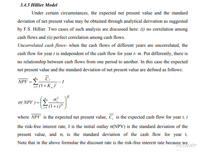
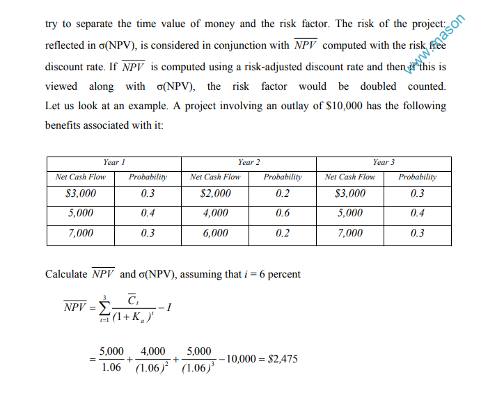
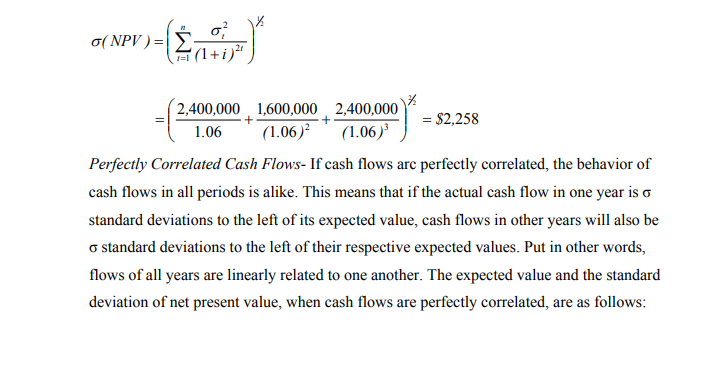
- Hillier model
- Simulation analysis
- Decision tree analysis
- Corporate risk analysis
3.4.1 Risk Adjusted Discount Rate Approach
The approach is based on the premise that the riskiness of a project may be accounted for by adjusting the discount rate (cost of capital). Relatively risky projects have relatively high discount rates while relatively safe projects have relatively low discount rates.
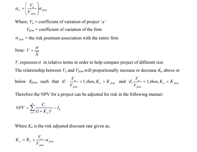
Remember CAPM which was expressed as: f m −+= RRRR f )( β , where the expected return was said to be function of the risk free rate plus a risk premium. This expression can be re expressed as follows: = RK +α afa
Where: Ka = the risk adjusted cost of capital for project a
Rf = the risk free rate
α a = the risk adjustment premium
As the risk increase so does α a and Ka such that, α a can be expressed as a function of the proportional relations between the standard deviation of the total firms cash flows i.e
3.4.2 Certainly Equivalent Approach
Proponents of this approach object to the use of a discount rate that lumps together the risk free rate and risk premium. They conclude that two important things account for the valuation process: time value of money and risk attitudes, which should be separated.
The decision rule associated with certainty equivalent approach is to undertake a project if its certainty equivalent NPV is greater than zero. Certainty equivalent of the cash flows Ct can be calculated in several ways some of these are:
- Reducing the cash flow estimate by a sufficient number of standard deviations to ensure that the occurrence will be certain under the normal distribution. This is done by reducing the cash flow estimates by 3 standard deviations (i.e. to be 99.72% certain that the occurrence will be at least equal to the certainty equivalent)
- Reducing the cash flow estimate by a factor “B” that reflects the financial manager’s willingness to trade the estimate for the certainty equivalent
- A time adjusted method where if the manager feels less certain of estimated cash flow over time, then B is reduced as the uncertainty of the future increases
3.4.3 Sensitivity Analysis
Since the future is uncertain, one may like to know what will happen to the viability of the project when some variable like sales or investment deviates from its expected value. In other words, you may want to do “what if” analysis or sensitivity analysis.
To understand the nature of sensitivity analysis, let us consider an example. Suppose you are the financial manager of Pembe Flour Mills. Pembe is considering setting up a new flour mill near Kitale. Based on Pembe previous experience, the project staff of Pembe
has developed the figures shown in Exhibit 13.2 (Note that the salvage value has assumed to be nil and the cost of capital to be 12 percent.)
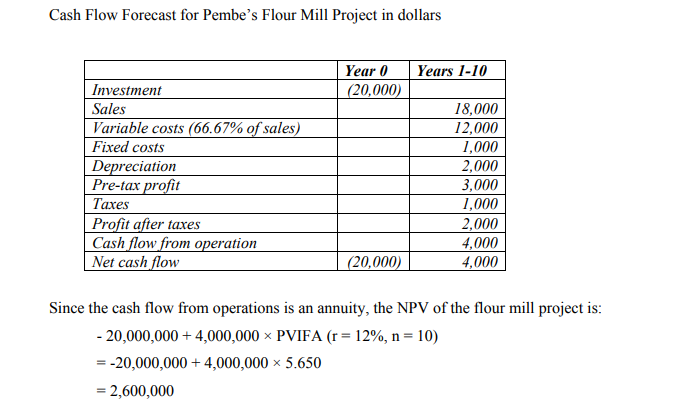
NPV based on the expected values of the underlying variables looks positive. You however, aware that the underlying variable can vary widely and hence you would like to explore the effect of such variations on the NPV. So you define the optimist and pessimistic estimates for the underlying variables. These are shown in the left hand co1umns of Exhibit the figure below. With this information, you can calculate the NPV for optimistic and pessimistic values of each of the underlying variables.
To do this, vary one variable at a time. For example, to study the effect of an adverse variation in sales (from the expected $18 million to the pessimistic $15 million), you maintain the values of the other underlying variables it their expected levels (This means the investment is held at $20 million, variable costs as a proportion of sales are held at 66.67 percent, fixed costs are held at $I million, so an and so forth.)
The NPV when the sales are at their pessimistic level and other variables at their expected level is shown on the right side of the above table. Likewise you can calculate the effect of variations in the values of the underlying variables. The NPVs for the pessimistic expected and optimistic forecasts are shown on the right side of the table Evaluation very popular method for assessing risk, sensitivity analysis has certain merits:
- It shows how robust or vulnerable a project is to changes in values of the underlying variables.
- It indicates where further work may be done. If the NPV is highly sensitive changes in some factor, it may be worthwhile to explore how the variability of the critical factor may he contained.
- It is intuitively very appealing as it articulates the concerns that project eva1uating normally have.
Notwithstanding its appeal and popularity, sensitivity analysis suffers from several shortcomings:
- It merely shows what happens to NPV when there is a change in some variable, without providing any idea of how likely that change will be.
- Typically, in sensitivity analysis only one variable is changed at a time. In the real world, however, variables tend to move together.
- It is inherently a very subjective analysis. The same sensitivity analysis may lead decision maker to accept the project while another may reject it. .
3.4.4 Scenario Analysis
Insensitivity analysis, typically one variable is varied at a time. In scenario analysis several variables are varied simultaneously. Most commonly three scenarios are considered: expected (or normal) scenario, pessimistic scenario and optimistic scenario and optimistic scenario. In the normal scenario all variables assume their normal values in the pessimistic scenario all the variables assume their pessimistic values and in the optimistic scenario all variables assume their optimistic values
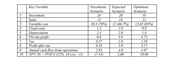
Scenario analysis may be regarded as an improvement over sensitivity analysis because it considers variations in several variables together.
However, scenario analysis has its own limitations:
It is based on the assumption that there are few well-delineated scenarios. This may not be true in many cases. For example, the economy does not necessarily lie in three discrete states, viz., recession, stability, and boom. It can in fact be anywhere on the continuum between the extremes. When a continuum is converted into three discrete states some information is lost.
Scenario analysis expands the concept of estimating the expected values. Thus, in a case where there are 10 inputs the analyst has to estimate 30 expected va1ues (3 ×10) to do the scenario analysis.
3.4.4 Break-even Analysis
In sensitivity analysis we ask what will happen to the project if sales decline or costs increase or something else happens. As a financial manager, you will also be interested in knowing how much should be produced and sold at a minimum to ensure that the project does not ‘lose money’. Such an exercise is called break even analysis and the minimum quantity at which loss is avoided is called the break-even point. The break -even point may be defined in accounting terms or financial terms. Accounting Break-even Analysis Suppose you are the financial manager of Pembe Mills is considering setting up a new flour mill near Kitale. Based on Pembe previous
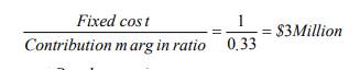
experience, the project staff of Pembe has developed the figures shown in the previous example. Note that the ratio of variable costs to sales is 0.667 (12/18). This means that every dollar of sales makes a contribution of $ 0.333. Put differently, the contribution margin ratio is 0.333.
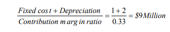
A variant of the accounting break-even point is the cash break-even point which is defined as the level of sales at which the firm neither makes cash profit nor incurs a cash loss. The cash break even sales is defined as:
Financial Break-even Analysis- The focus of financial break-even analysis is on NPV and not on accounting profit, at what level of sales will the project have a zero NPV? To illustrate how the financial break-even level of sales is calculated, let us go back to
Pemble mill project. The annual cash flow of the project depends on sales as follows:
Variable costs: 66.67 percent of sales
Contribution: 33.33 percent of sales
Fixed costs: $ 1 million
Depreciation: $ 2 million
Pre-tax profit: 0.333 × Sales) – $ 3 million
Tax (at 33.3%) 0.333 (0.333 Sales – $ 3 million)
Profit after tax .667 (0.333 x Sales -$ 3 million)
Cash flow (4 + 7): Es. 2 million + .667 (0.333 × Sales – $ 3 million)
= 0.222 Sales
Since the cash flow lasts for 10 years, its present value at a discount rate of 12 percent is:
PV (cash flows) = 0.222 Sales × PVIFA (10 years, 12%)
= 0.222 Sales z 5.65(1
= 1.254 Sales
The project breaks even in NPV terms when the present value of these cash flows equals
the initial investment of Es. 20 million. Hence, the financial break-even occur, when
PV (cash flows) = Investment
1.254 Sales = $ 20 million
Sales = $ 15.95 million
Thus, the sales for the flour null must be $15.95 million per year for the investment to have a zero NPV. Note that this is significantly higher than $ 9 million which represents the accounting break-even sales
3.4.6 Simulation Analysis
Sensitivity analysis indicates the sensitivity of the criterion of merit (NPV, IRR, or any other) to variations in basic factors and provides information of the following type: If the quantity produced and sold decreases by 1 percent, other things being equal, the
NPV falls by 6 percent. Such information, though useful, may not he adequate for decision making. The decision maker would also like to know the likelihood of such occurrences. This information can be generated by simulation analysis which may be used for developing the probability profile of a criterion of merit by randomly combining values of variables which a bearing on the chosen criterion.
Procedure- The steps involved in simulation analysis are as follows:
1. Model the project. The model of the project shows how the net present value is related to the parameters and the exogenous variables. (Parameters are input variables specified by the decision maker and hold constant over all simulation runs. Exogenous variables are input variables which are stochastic in nature and outside the control of the decision maker).
2. Specify the values of parameters and the probability distributions of the exogenous variables.
3. Select a value, at random, from the probability distributions of each of the exogenous variables.
4. Determine the net present value corresponding to the randomly generated values of exogenous variables and pre-specified parameter values.
5. Repeat steps (3) and (4) a number of times to get a large number of simulated net present values.
6. Plot the frequency distribution of the net present value.
In real life situations, simulation is done only on the computer because of the computational tedium involved. However, to give you an idea of what goes on in simulation, we will work with a simple example where simulation ha been done manually. Pharma Chemicals is evaluating an investment project whose net present value has been modelled as follows:
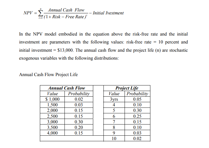
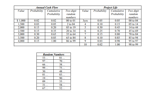
The firm wants to perform 10 manual simulation runs for this project. To perform the simulation runs, we have to generate values, at random, for the two exogenous variables: annual cash flow and project life. For this purpose, we have to (i) set up the correspondence between the values of exogenous variables and random numbers, and (ii) choose some random number generating device. The table below shows the correspondence between various variables and two digit random numbers. The table presents a table of random digits that will be used for obtaining two digit random numbers.
Now we are ready for simulation. In order to obtain random numbers from the table, we may begin anywhere at random in the table and read any pair of adjacent columns (since we are interested in a two-digit random number) and read column-wise or row-wise.
For our example, let us use the first two columns of the table. Starting from the top, will read down the column. For the first simulation run we need two, two-digit random numbers, one for the annual cash flow and the other for the project life. These
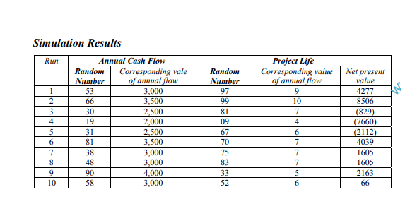
numbers are 53 and 97 and the corresponding values for annual cash flow and project life are $3,000 and 9 years respectively. We go further in this manner. The table shows the random numbers so obtained and the results of simulation
Evaluation An increasingly popular tool of risk analysis, simulation offers certain advantages:
- Its principal strength lies in its versatility. It can handle problems characterized by numerous exogenous variables following any kind of distribution, and complex interrelationships among parameters, exogenous variables, and endogenous variables. Such problems often defy the capabilities of analytical methods.
- It compels the decision maker to explicitly consider the interdependencies and uncertainties characterizing the project.
Simulation, however, is a controversial tool which suffers from several shortcomings:
- It is difficult to model the project and specify the probability distributions of exogenous variables.
- Simulation is inherently imprecise. It provides a rough approximation of the prob. ability distribution of net present value (or any other criterion of merit). Due to imprecision, the simulated probability distribution may be misleading when a tail the distribution is critical.
- A realistic simulation model, likely to be complex, would most probably be constructed by a management scientist, not the decision maker. The decision maker lacking understanding of the model, may not use it.
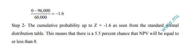
- To determine the net present value in a simulation run the risk-free discount rate used. This is done to avoid prejudging risk which is supposed to be reflected in they dispersion of the distribution of net present value. Thus the measure of net present value takes a meaning, very different from its usual one that is difficult to interpret
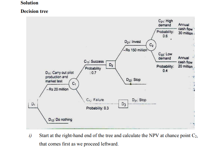
3.4.7 Decision Tree Analysis
To analyze such situations where sequential decision making is involved decision tree analysis is helpful.
The key steps in decision tree analysis are a follows:
Delineate the decision tree
Evaluate the alternatives
Delineate the Decision- Tree Exhibiting the anatomy of the decision situation, the decision e shows:
The decision points (typically represented by squares), the alternative options available for experimentation and action at these points, and the investment outlays associated with these options.
The chance points (typically represented by circles) where outcomes are dependent on the chance process, the likely outcomes at these points along with the probabilities thereof, and the monetary values associated with them.
Evaluate the Alternatives- Once the decision tree is delineated and data about probabilities and outcomes gathered, decision alternatives may be evaluated as follows:
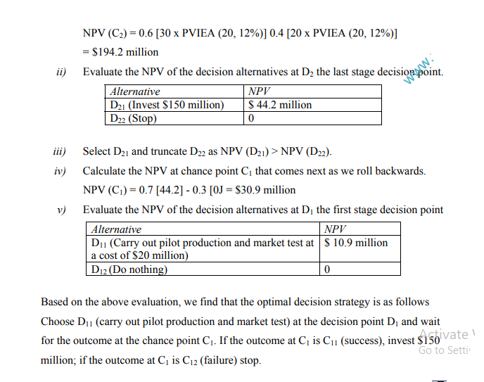
- Start at the right-hand end of the tree and calculate the NPV at various chance points that come first as you proceed leftward.
- Given the NPVs of chance points in step 1, evaluate the alternatives at the final stage decision points in terms of their NPVs.
- At each final stage decision point, select the alternative which has the highest NPV and truncate the other alternatives. Each decision point is assigned a value equal to the NPV of the alternative selected at that decision point.
- Proceed backward (leftward) in the same manner, calculating the NPV at chance points, selecting the decision alternative which has the highest NP at various decision points, truncating inferior decision alternatives, and assigning NPVs to decision points, till the first decision point is reached.
Illustration
General electric have come up with an electric cycle. The firm is ready for pilot production and test marketing. This will cost $20 million and take few weeks. Management believes that there is a 70 percent chance that the pilot production and test marketing will be successful. In case of success, G.E. can build a plant costing $150 million very quickly. The plant will generate an annual cash inflow of $30 million for 20 if the demand is high or an annual cash inflow of $21million if the demand is moderate. High demand has a probability of 0.6; moderate demand has a probability 0.4. Start at the right-hand end of the tree and calculate the NPV at chance point C, that comes first as we proceed leftward. Advice G.E. on the best course of action
3.4.8 Corporate Risk Analysis
A project’s corporate risk is its contribution to the overall risk of the firm. Put differently, it reflects the impact of the project on the risk profile of the firm’s total cash flows. On a stand-alone basis a project may be very risky hut if its returns are not highly correlated or, even better, negatively correlated-with the returns on the other projects its corporate risk tends to be low. Aware of the benefits of portfolio diversification, many firms consciously pursue a strategy diversification. Unilever Limited, for example, has a diversified portfolio comprising, in the main, of the following businesses: soaps and detergents, personal care products, food, and tea.
The proponents of diversification argue that it helps in reducing the firm’s overall risk exposure. As most businesses are characterized by cyclicality it seems desirable that there two to three different lines of business in a firm’s portfolio. The logic of corporate diversification for reducing risk, however, has been questioned. Why should a firm diversify when shareholders can reduce risk through personal diversification? All that they have to do is to hold a diversified portfolio of securities or participate in a mutual fund scheme. Indeed, they can do it more efficiently.
There does not seem to be an easy answer. Although shareholders can reduce risk through personal diversification there are some other benefits from corporate diversification. Stable earnings and cash flows enable a firm to attract talent, to secure commitment from various stakeholders, to exploit tax shelters fully, and to check adverse managerial incentives